16 Evaluating Regression Models
To this point we’ve concentrated on the nuts and bolts of putting together a regression, without really evaluating whether our regression is good. In this chapter we’ll turn to that question, both with regards to whether a linear regression is the right approach to begin with, but also ways to think about how to determine whether a given independent variable is useful. We’ll start by adding more depth to the types of regression we’ve used in previous chapters.
16.1 Concepts
The code used in the Concepts section of this chapter can be viewed here and copied into R to process. You may need to install additional packages for the code to work.
16.1.1 Ordinary least squares
Regression analysis is a broad class of analytic techniques. What we’ve practiced in the last few chapters is a specific type of regression, specifically ordinary least squares (OLS). It’s called ordinary least squares because the coefficients in an OLS regression are chosen by the principle of least squares. As we’ve already said, our regression coefficient (or the slope of our line) is chosen to minimize the difference between the predicted and the observed values. That can also be stated as minimizing the sum of the squared distances: we choose the slope in order to minimize the distanced between the predicted value of y by our line and the actual value of y in our data. Let’s look at that idea visually.
We’ll use two made up variables for this analysis, so don’t worry about what is on either axis.
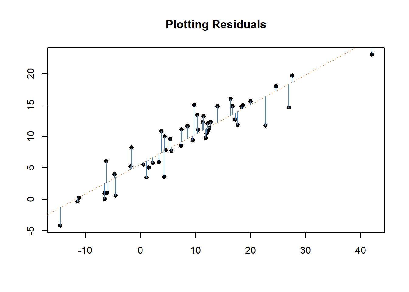
The blue lines above show how far our prediction missed for each point in the regression. Ordinary least squares regression works to minimize the amount that our model misses in total. It could adjust the orange line (the line of best fit) to reduce how far off it is on the biggest misses, but that would increase the total error across all the other points.
So, to state it a different way, in OLS the regression line is the line that achieves the least square criterion, whereby the sum of squared distances between the predicted and observed values are minimized. But in order for an OLS regression to be appropriate we have to assess whether 4 critical assumptions are met. This chapter is going to be devoted to discussing the following 4 assumptions, how to test for those 4 assumptions, and what is going on in our model that might make it violate these assumptions. Some fixes to correct for violations can be done within an OLS regression and future chapters will address more significant changes we may need to make to our models. In addition, this chapter will discuss a few additional metrics we have to decide whether to include additional Independent variables, and how to evaluate the overall fit of our model.
The four assumptions are:
- Linearity, the relationship between y and x is linear.
- Independent, each observation is independent.
- Homoscedasticity, the residuals have constant variance at every level. This is known as homoscedasticity.
- Normality, the residual errors are normally distributed.
All of these assumptions have to do mostly with the residuals of our model. When we run a regression it is human instinct to look at the coefficients and whether our variables were significant or not. That’s natural, but what is actually more important is what we’re not explaining with our independent variables. It’s what we miss that tells us whether our model is performing well.
16.1.2 Assumption 1: Linearity
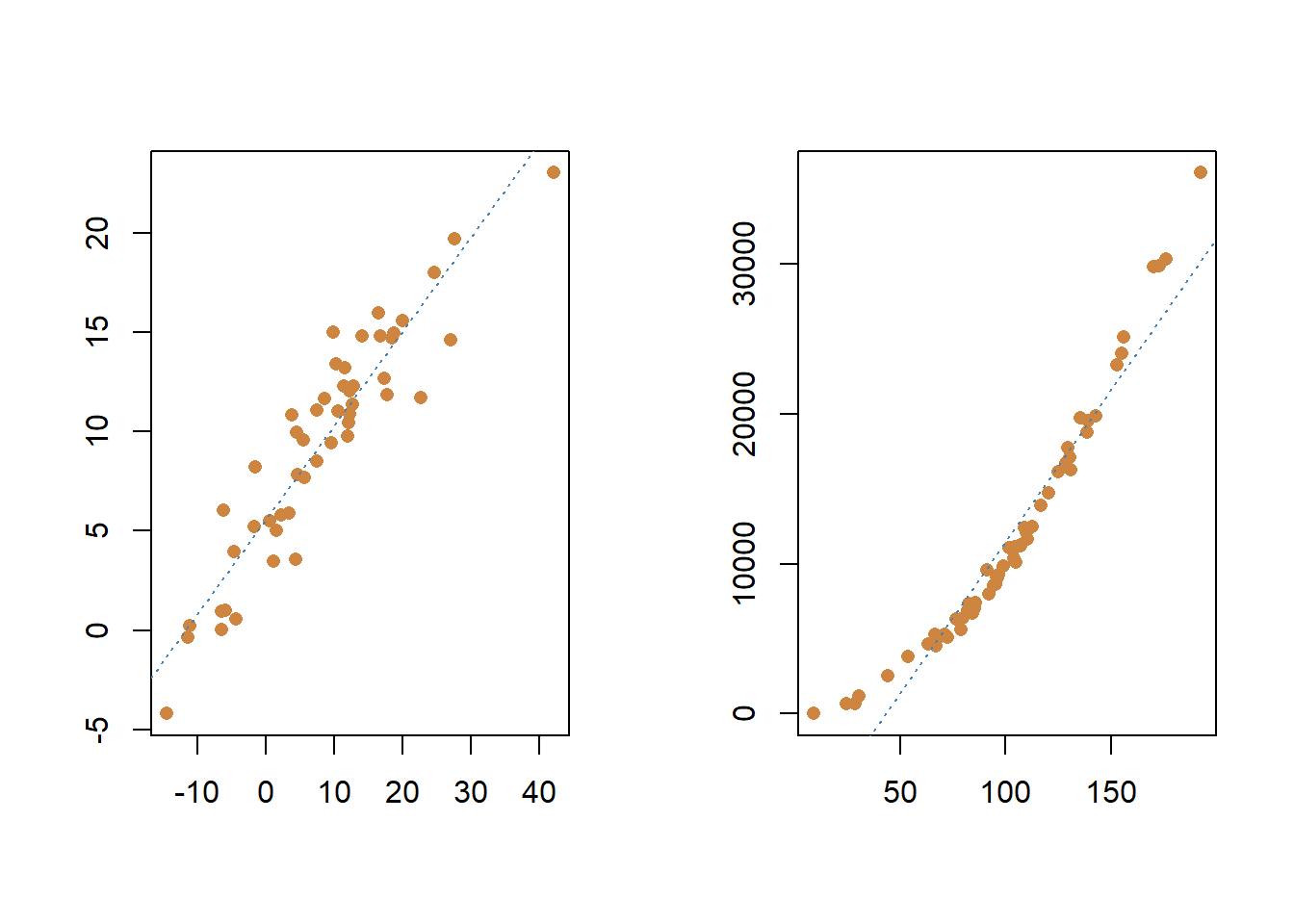
If you’re using a linear regression, the relationship between your variables needs to be linear. Sometimes a straight line does minimize the distance between our predictions and the true values, but that wont always be the case. You can often test that assumption just by looking at a simple plot of the two variables, as we’ve done before. For instance, you can see the linear relationship in the two variables I used in the above example, but the plot on the right appears to be non-linear. The values for y first decline as x increases and approaches 0, then y and x both increase after x gets above 0.
##
## Call:
## lm(formula = y2 ~ x2)
##
## Residuals:
##     Min      1Q  Median      3Q     Max
## -2424.8 -1501.2  -699.6   717.7  6893.3
##
## Coefficients:
##              Estimate Std. Error t value Pr(>|t|)
## (Intercept) -8720.891    787.854  -11.07 6.29e-16 ***
## x2            202.277      7.214   28.04  < 2e-16 ***
## ---
## Signif. codes:  0 '***' 0.001 '**' 0.01 '*' 0.05 '.' 0.1 ' ' 1
##
## Residual standard error: 2118 on 58 degrees of freedom
## Multiple R-squared:  0.9313, Adjusted R-squared:  0.9301
## F-statistic: 786.3 on 1 and 58 DF,  p-value: < 2.2e-16
Our independent variable is significant, so what’s the big issue? Our coefficient is supposed to be telling us the change that we’ll observe in the dependent varaible based on changes in the independent - when the relationship isn’t linear, that value becomes unreliable. If we only evaluate our coefficient and p-value, we’re ignoring all the information we’re not capturing with that line; a straight line isn’t a very good approximation of the true relationship in our data. What we’re missing is that the residuals are very large in some cases, particularly for the small and large values of the independent variable. The middle values for x are pretty close to the line, but the lowest and highest value for x get further and further away from our predictions.
One typical way to test if the relationship between your dependent and independent variables is linear is by graphing the residuals from the model against the predicted values. What we want to see is that the model doesn’t miss with any specific pattern. We know the line wont perfectly capture each individual point, but we’d like it miss as much for low and medium and high values of the independent values. In general, the values should be evenly split above and below 0. Let’s graph that for both of the sets of data we’ve looked at earlier in this chapter.
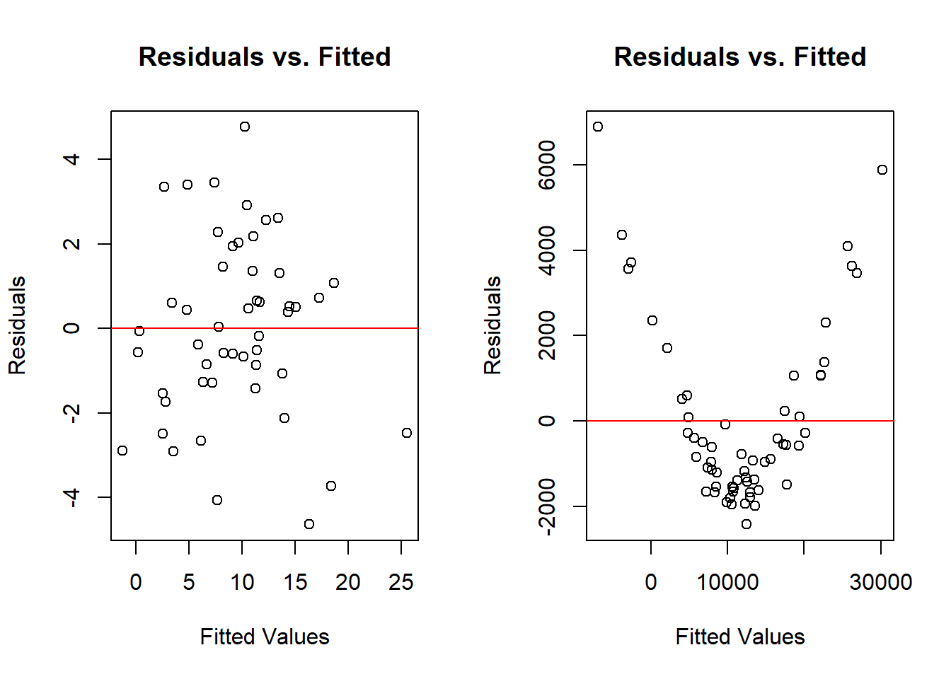
Again, the residuals are how far off each guess is at the value of y, and the x is what we predicted the value of y to be. What we want to observe is that the values are randomly distributed around the horizontal line at 0. What the graph on the right shows us shows is that the residuals were really high for the observations that were predicted to have the highest or lowest values in the data. The fact those all had positive residuals means the line predicted values that were too low for those observations. Alternatively. The line predicted too high of values for the middle set of observations, but those misses were at least smaller. The first model is pretty balanced above and below the red line, so it appears that relationship is linear.
We can only really visualize the relationship between one independent variable and our dependent variable, but we can graph the residuals and the fitted values no matter how many independent variables. As such, it’s a better technique to get comfortable with in evaluating whether your model is linear.
So that’s the first assumption, that the data between our independent and dependent variables is best modeled using a linear relationship. There’s plenty we can do when that isn’t the case, it just means we need to adjust our data a little bit. But that’s a problem for another section.
16.1.3 Assumption 2: Independence
We assume that each observation in our data is collected independently and isn’t dependent on any other observation in our data. A great example of data that will achieve independence is something collected using a simple random sample. Why wouldn’t the data be independent? A common violation of that assumption comes from when data is collected for individuals or units at multiple points in time.
Let’s say I’m interested in studying how graduates from my university do in life financially. I take a sample of graduates from the university and ask them what their major was and track their current salary. One participates name is Sally, and if I do the same survey a year later with the same people, how much do you think Sally’s salary will have changed? She might have gotten promoted or a raise or lost her job. It’s possible that it changed, but across the entire sample most people’s salaries in the second year could be predicted pretty well by their salary a year earlier. The two observations of salary aren’t independent. We’ll discuss strategies for dealing with that later, but there wont be a chapter on that section in this book for a while. If you’re interested, this is a useful (though somewhat barebones guide).
16.1.4 Assumption 3: Homoscedasticity
Here I need to add something, or make something explicit, that we’ve skipped over to this point. We haven’t fully talked about how to write out a regression model yet. That hasn’t been too important, but at this point I need to discuss that in order to have assumption 3 make sense. And we’re going to have to write a little bit of Greek here, because that’s the way that mathematicians like to write things so that people don’t realize how simple their equations actually are.
In a regression model with one independent variable, the regression model would be said to consist of four terms.
There’s the dependent variable, on the left side of the equation. On the right side there is the constant (the x-intercept), the independent variable, and an error term. If we were to write out a proper formal looking regression model it might look like this:
\(Y\) = \(\beta_{0}\) + \(\beta_1 X_{1}\) + \(\epsilon\)
Where Y is our dependent variable or outcome \(\beta_{0}\) is our constant or x-intercept \(\beta_{1}\) is the coefficient for our independent variable \(X_{1}\) is the value of our independent variable and \(\epsilon\) is the error term.
And if we had 3 independent variables, this is what it would look like:
\(Y\) = \(\beta_{0}\) + \(\beta X_{1}\) + \(\beta X_{2}\)+ \(\beta X_{3}\) + \(\epsilon\)
Where Y is our dependent variable or outcome \(\beta_{0}\) is our constant or x-intercept \(\beta_{1}\) is the coefficient for our first independent variable \(X_{1}\) is the value of our first independent variable \(\beta_{2}\) is the coefficient for our second independent variable \(X_{2}\) is the value of our second independent variable \(\beta_{3}\) is the coefficient for our third independent variable \(X_{3}\) is the value of our third independent variable and \(\epsilon\) is the error term.
What does the error term mean? We don’t expect that our regression models will perfectly predict Y. Well, the error term captures the amount of variability in the dependent variable that is not explained by our independent variable. That might sound a lot like the residuals we described earlier, but there is a slight distinction. Although the terms are sometimes used synonymously, error terms are unobservable while residuals are observable (we measured them above for instance). The error term represents the way that the observed data in our sample differs from the actual population, while residuals represent the way the observed data differs within the sample data. It’s a really small, but important distinction.
How can we check that? We can do that with a test in R called the Breush-Pagan test. I don’t want to get into the details on the Breush-Pagan and how it does what it does, but what it does is test whether the variance of the error term for a regression are constant. The null hypothesis of the test is that our error terms are homoscedastic (which is good!). We don’t want to reject the null hypothesis here. The alternative is that our error term is heteroscedastic, which means we need to adjust our model.
When I run that test with the data that was graphed on the left (the actually linear data), I get a p-value of .31. A p-value of .31 is well above the .05 cutoff for rejecting the null hypothesis. That’s great, our error term was homoscedastic for that model. I’ll show you how to run that test yourself later in the Practice section.
We can also visualize the variance of the error terms. What you’ll see is that the errors are fairly randomly distributed across the fitted values of the regression, which means there isn’t a clear pattern to where the errors are occurring. It’s not perfect, but what’s important is that we don’t see any clear violation of our assumption.
What would we need to do if there was heteroscedasticity in the model? Most likely, we’d need to add more independent variables to help explain the issues that are making our errors larger in some cases than others.
For instance, let’s say we’re testing the effect of studying on grades on a final in an introductory math class. In general, students that studied more did better on the test, but the variance is very high for students that didn’t study very much - some did well, others did very poorly. The error term isn’t constant in that case. What we would need to do is figure out what could help us explain the difference in performance for those students that didn’t study very much? Maybe they cheated, or perhaps they’d taken the class in a previous semester and their credits didn’t transfer, or something else. Regardless, a part of our dependent variable is being consistently under-explained, so we are likely missing independent variables to help understand that portion of the variance. We’ll talk more later in this chapter about how to choose when including or excluding independent variables.
16.1.5 Assumption 4: Normality
Our final assumption is that the residual errors from our model are normally distributed. What does normally distributed mean? We learned about normal distributions in an earlier chapter, but broadly it refers to a distribution of data that falls evenly above and below the mean in a bell shape. in the case of regression, we want to know that our model is off sort of evenly for all of the different values. Some will have an outcome that is predicted too high, others too low, but our model isn’t consistently under-predicting every value of the dependent variable.
We can check that with a histogram for our regressions.
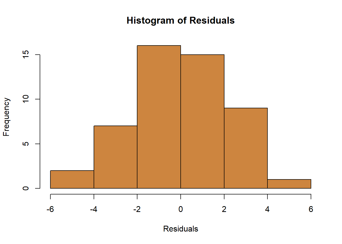 It’s not a perfect bell shape, but it’s close. And considering that we only have 50 observations in our data, it’s a pretty good approximation of evenly split above and below 0.
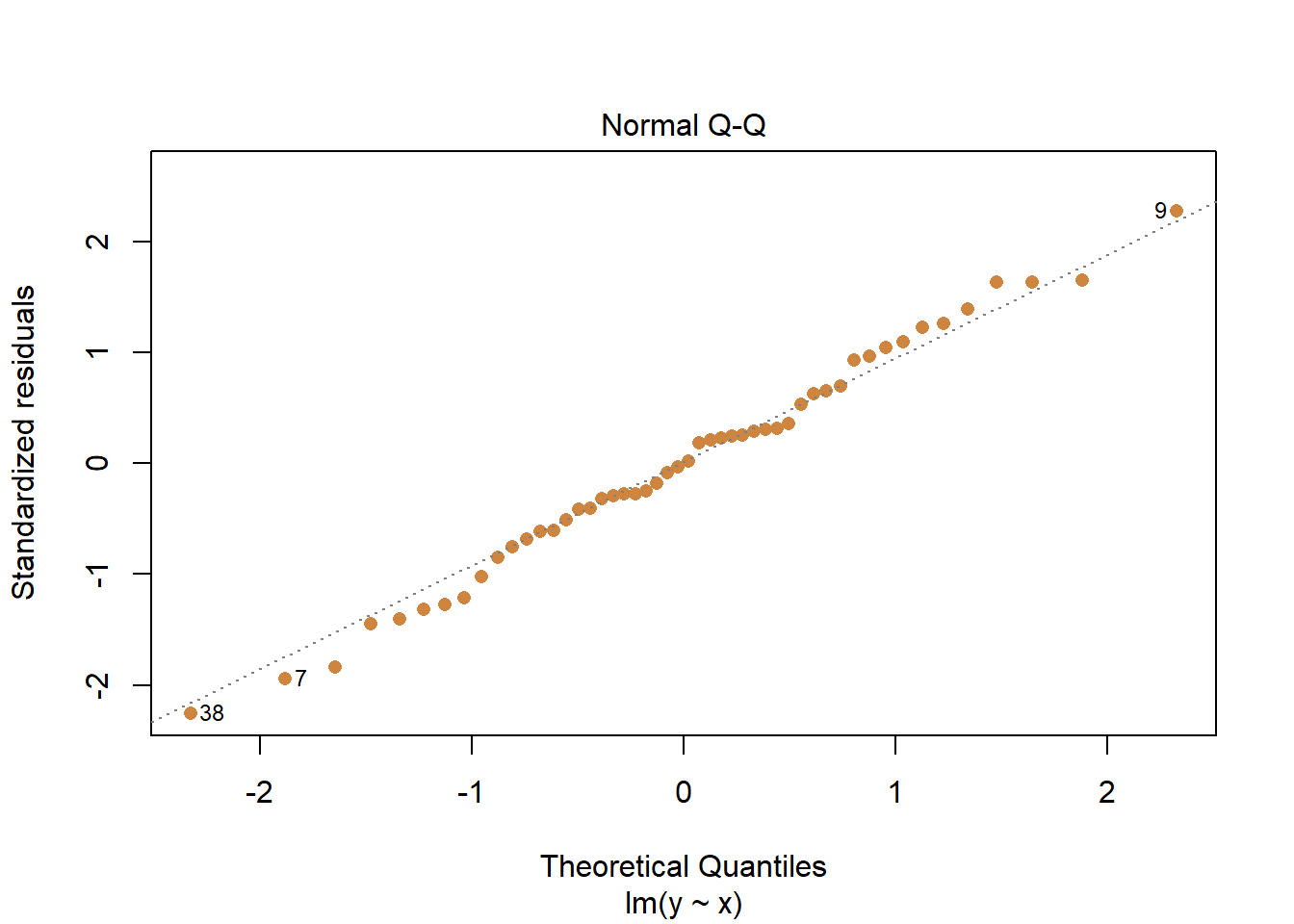
Or we can use what’s called a Q-Q Plot, which plots the quantiles for the fitted values of the regression against a standardized set of residuals. You don’t entirely need to understand what that means to appreciate that what you want to see is a close match between the points and the 45 degree line. In the case below, we can again see the residuals are normal distributed.
16.1.6 Model evaluation
The 4 assumptions described above help us to make sure that our regression results are appropriate and reliable. But we also want to ask whether our regression analysis is valuable as a tool for understanding the phenomena we’re studying. This section will focus on some of the tests and metrics that are available to you in choosing whether to include certain variables and how to evaluate whether your model has performed well at predicting your dependent variable.
16.1.6.1 R-Squared
A prominent metric for evaluation your model is the R-Squared or \(R^{2}\). R-Squared can range from 0 to 1, and is commonly interpreted as indicating the percentage or share of the variance in the dependent variable that is explained by your model. Specifically, it is calculated as:
\(R^{2}\) = 1- \(\frac{Total Variation}{Unexplained Variation}\)
Higher values of \(R^{2}\) are preferred, because they indicate we’ve explained more of the variation in our dependent variable. We’ve done a better job of predicting our outcome.
It should be noted though that R-Squared will never decrease with the addition of new variables to our model. So that means we should just always add new variables, and our model will always be better, right? Not exactly. And there’s multiple reasons we don’t want to just add variables without any reason. But for that reason, because R-Squared will always increase (even if insignificantly), the adjusted R-Squared is generally a preferred metric for model evaluation.
The adjusted R-Squared adjusts for the addition of multiple variables. It will increase as additional independent variables improve the fit of the model, but it’ll also decrease if independent variables don’t improve the fit of the model more than chance would expect. It should be emphasized, they’re generally going to be similar, but the adjusted R-Squared will typically be a little smaller. You’ll get both with the default regression output in R. Let’s look at that for a regression for wages, similar to what we did in the chapter on Multiple Regression
##    experience weeks occupation industry south smsa married gender union
## 1           9    32      white      yes   yes   no     yes   male    no
## 2          36    30       blue      yes    no   no     yes   male    no
## 3          12    46       blue      yes    no   no      no   male   yes
## 4          37    46       blue       no    no  yes      no female    no
## 5          16    49      white       no    no   no     yes   male    no
## 6          32    47       blue      yes    no  yes     yes   male    no
## 7          21    48       blue       no    no   no     yes   male   yes
## 8          29    51       blue      yes    no  yes     yes   male   yes
## 9           9    48      white       no   yes  yes     yes   male    no
## 10          9    40      white       no   yes  yes     yes   male    no
## 11         30    47       blue       no    no  yes     yes   male   yes
## 12         27    46       blue       no   yes  yes     yes   male   yes
## 13         32    46       blue       no   yes  yes     yes   male    no
## 14         21    44      white       no   yes  yes     yes   male    no
## 15         15    48      white       no    no   no      no female    no
## 16         22    49       blue       no   yes  yes      no female    no
## 17         22    47      white      yes    no   no     yes   male    no
## 18         31    47      white      yes   yes  yes     yes   male    no
## 19         46    40       blue      yes    no  yes     yes   male   yes
## 20         31    48      white      yes    no   no     yes   male    no
## 21         34    42       blue      yes   yes   no     yes   male   yes
## 22         26    47      white       no    no   no     yes   male    no
## 23         17    50      white       no    no  yes     yes   male    no
## 24         11    50       blue       no    no   no      no female    no
## 25         14    41      white       no    no  yes     yes   male   yes
## 26         20    48      white      yes   yes  yes     yes   male    no
## 27         14    23      white       no    no   no      no   male    no
## 28         32    49       blue       no    no  yes     yes   male    no
## 29         37    49      white       no    no  yes     yes   male    no
## 30         23    49      white       no   yes  yes      no female    no
## 31         28    45      white      yes    no  yes     yes   male    no
## 32         36    47      white      yes    no  yes     yes   male    no
## 33         20    49      white       no    no  yes     yes   male    no
## 34         51    46       blue       no   yes   no     yes   male    no
## 35         14    45       blue      yes    no  yes     yes   male   yes
## 36         21    41      white       no   yes  yes     yes   male    no
## 37         18    49      white       no    no  yes      no   male    no
## 38         16    49       blue      yes    no   no     yes   male   yes
## 39         12    51      white       no    no  yes     yes   male    no
## 40         36    47      white       no   yes   no     yes   male   yes
## 41         26    47      white       no   yes  yes     yes   male    no
## 42         36    49       blue      yes    no  yes      no female   yes
## 43         11    49      white       no    no  yes     yes   male    no
## 44         13    46      white      yes    no  yes     yes   male    no
## 45         19    49      white       no    no  yes      no female    no
## 46         12    47       blue       no    no   no     yes   male   yes
## 47         32    48      white       no    no  yes     yes   male    no
## 48         32    49      white      yes    no  yes      no   male    no
## 49         37    48      white      yes    no   no     yes   male    no
## 50         37    28      white       no    no  yes      no female   yes
## 51         37    44      white      yes    no  yes     yes   male    no
## 52         31    49      white       no    no  yes     yes   male   yes
## 53         19    48      white       no    no   no     yes   male    no
## 54         19    50       blue      yes    no   no     yes   male   yes
## 55         38    46       blue      yes    no  yes     yes   male   yes
## 56         29    50       blue      yes   yes   no     yes   male    no
## 57         27    48      white       no   yes  yes     yes   male    no
## 58         43    48       blue      yes    no  yes     yes   male    no
## 59         32    46      white      yes    no  yes     yes   male    no
## 60         24    43       blue       no    no  yes      no female   yes
## 61         30    26      white       no    no  yes      no female    no
## 62         13    49       blue      yes   yes   no     yes   male    no
## 63         17    50      white       no    no   no     yes   male    no
## 64         40    50       blue      yes    no  yes     yes   male    no
## 65         36    45       blue      yes    no  yes     yes   male   yes
## 66         26    48       blue      yes   yes   no     yes   male    no
## 67         34    49       blue       no   yes   no     yes   male    no
## 68         40    46       blue      yes    no  yes     yes   male   yes
## 69         33    48       blue      yes    no  yes     yes   male    no
## 70         14    48      white       no    no   no     yes   male    no
## 71         13    48      white       no   yes  yes      no   male    no
## 72         17    42      white       no    no   no     yes   male   yes
## 73         19    47      white       no    no  yes     yes   male   yes
## 74          9    52       blue       no   yes   no      no   male    no
## 75         29    47       blue      yes   yes   no     yes   male    no
## 76         15    49       blue       no    no   no     yes   male    no
## 77         16    39       blue       no   yes   no     yes   male    no
## 78         43    50       blue       no   yes  yes      no   male    no
## 79         16    50       blue       no    no   no      no female    no
## 80         11    50      white      yes    no   no     yes   male    no
## 81         12    50       blue       no    no  yes     yes   male    no
## 82         28    36       blue       no   yes   no     yes   male   yes
## 83         18    46       blue       no    no  yes      no   male   yes
##    education ethnicity wage
## 1          9     other  515
## 2         11     other  912
## 3         12     other  954
## 4         10      afam  751
## 5         16     other 1474
## 6         12     other 1539
## 7         12     other  680
## 8         10     other  984
## 9         16     other 1350
## 10        16     other  845
## 11        12     other 1400
## 12        12     other 1156
## 13        12     other 1636
## 14        17     other 1240
## 15        14     other  650
## 16        12      afam  595
## 17        14     other 1250
## 18        16     other 2450
## 19        12     other 1029
## 20        16     other 1432
## 21         4     other  628
## 22        14     other 1150
## 23        16     other 2680
## 24        12     other  350
## 25        17     other 1000
## 26        15     other 1583
## 27        16     other 1500
## 28        12     other  850
## 29        14     other 1920
## 30        12     other  768
## 31        17     other 2025
## 32        16     other 2300
## 33        16     other 1750
## 34         8     other  397
## 35        13      afam 1125
## 36        10     other 1313
## 37        14     other 1651
## 38        12     other  680
## 39        13     other  905
## 40         8     other 1569
## 41        16     other 2310
## 42        12      afam 1125
## 43        16     other 1700
## 44        17     other 2000
## 45        13     other  775
## 46        12     other  700
## 47        14     other 1200
## 48        16     other 1700
## 49        16     other 2492
## 50        12     other  943
## 51        17     other 2750
## 52        16     other 2100
## 53        13     other 1350
## 54        11     other 1212
## 55         8     other 1350
## 56        12     other  688
## 57        11     other  552
## 58        14     other 1250
## 59        17     other 2100
## 60        11      afam  479
## 61        17     other 1250
## 62        16     other 1440
## 63        17     other 1582
## 64        12     other  900
## 65         8     other 1148
## 66         8     other  950
## 67        12     other  650
## 68        12     other 1050
## 69        13     other 1023
## 70        16     other 1300
## 71        16     other 1639
## 72        17     other 1100
## 73        16     other 1228
## 74        13     other  350
## 75         8      afam  630
## 76        13     other  516
## 77        10     other  534
## 78        12     other  550
## 79         8     other  425
## 80        17     other 1425
## 81        16     other 1304
## 82        12     other 1171
## 83        12     other  709
##  [ reached 'max' / getOption("max.print") -- omitted 512 rows ]
##
## Call:
## lm(formula = wage ~ ethnicity + occupation + experience + married,
## data = PSID1982)
##
## Residuals:
## Min 1Q Median 3Q Max
## -1029.1 -310.9 -37.3 201.0 3675.0
##
## Coefficients:
## Estimate Std. Error t value Pr(>|t|)
## (Intercept) 1015.014 58.907 17.231 < 2e-16 ***
## ethnicityafam -209.455 76.645 -2.733 0.00647 **
## occupationblue -401.977 38.774 -10.367 < 2e-16 ***
## experience 4.706 1.818 2.588 0.00990 **
## marriedyes 306.413 50.548 6.062 2.4e-09 ***
## ---
## Signif. codes: 0 '***' 0.001 '**' 0.01 '*' 0.05 '.' 0.1 ' ' 1
##
## Residual standard error: 468.9 on 590 degrees of freedom
## Multiple R-squared: 0.2256, Adjusted R-squared: 0.2203
## F-statistic: 42.97 on 4 and 590 DF, p-value: < 2.2e-16We got an adjusted R-Squared of .22, which means we explained about 22% of the variation in wages. How should we feel about that?
The strength of R-Squared is in its simplicity because the interpretation (how much of our variation did we explain?) is fairly easy to intuit. However, it should be emphasized that there’s no rule about what a good R-Squared value is. Yes, the higher the better, but comparing them across different models with different dependent variables can be difficult. Somethings like height can be easy to predict accurately, particularly if you have your choices of independent variables. If I knew the heights of a person’s parents, their shoe size, and their weight, I’ll bet I could explain almost all the variation in height, and I’d get a really high R-Squared. But other things, like predicting someone’s income, would be a lot noisier. I’d end up with a really low R-Squared, even though I might do better and more creative work in trying to predict that.
That’s why R-Squared and adjusted R-Squared are generally emphasized in an introductory stats class. That said, most journal articles shy away from using it as a metric of model quality. In part that’s because it isn’t appropriate for some different types of models (more on that in a different section), but a lot of that has to do with some more complicated statistical argument, which you can find elsewhere. I think part of the issue is because R-Squared was used too much because it was easy to understand. People started interpreting it as a measure of goodness-of-fit, for how well your regression line fit the data. But that’s incorrect, if you scroll all the way back up to look at the regression results for the relationship that violated our assumption of linearity, the adjusted R-Squared was 0.9401. That’s a really good R-Squared, for a model that is inappropriate! So remember, R-Squared is just a measure of how much variation the model explains, it says nothing about whether your model is correct. And don’t be surprised if you keep working with data that at some point someone is going to be a prick about you using R-Squared to evaluate your model.
16.1.6.2 Akaike Information Criterion
There are other metrics that can be used to evaluate the overall fit of your model. A common one is the Akaike information criterion (AIC), which measures how well your model fits the data, but also carries a penalty for how many independent variables you include. As such, it balances the goodness-of-fit of your model with its simplicity. In other words, AIC deals with both the risk of over-fitting and the risk of under fitting. It’s an ideal metric to look at when comparing different models with the same dependent variable, because it’ll give you a straightforward assessment of whether more independent variables improve the model. However, like R-Squared, it can be difficult to use when comparing models with different dependent variables. With AIC, lower values indicate a better model, and values can be negative.
AIC is calculated by using the residual sum of squares. The residual sum of squares (RSS) is the sum of the squared distances between your actual versus your predicted values. Squaring the residuals penalizes larger residuals (a residual of 1 stays 1, a residual of 2 becomes 4, a residual of 3 becomes 9…).
We multiply the log of the residual sum of squares by the number of observations in your data (n), and add the number of independent variables (m) multiplied by 2.
AIC = n * log(RSS) + 2m
You don’t need to calculate that by hand though, R has a command to do it for you. I only provide the formula to help understand the intuition of how it balances adding additional independent variables against improving the fit of the model.
You’ll see a few other metrics pop up in regression output commonly.
One is the residual standard error (RSE). The RES is a measure of the variability of the residuals from the model. Residual standard error looks at how far each point is from the predicted value, squares that number and divides it by the degrees of freedom. Your degrees of freedom are the number of observations you have in your data, minus the number of independent variables you are including in your model. For RSE, the closer your number is to 0 the better. I don’t think it’s a better or worse metric than AIC or R-Squared, it’s just another way of evaluating your model.
Finally, there’s the F-Statistic, which in my opinion isn’t that useful. The F-test tests whether any of the independent variables in a regression model are significant, or more specifically whether they significantly improve your ability to predict the dependent variable. But, we already know that if any of our independent variables is significant. And once you include multiple independent variables, it’s almost inevitable that they’ll collectively improve your ability to understand the dependent variable, even if non are significant. You can compare the F-statistics across models, but there are other metrics for that. Just wanted to explain that, since it’ll pop up in regressions and now you’ll know why you don’t really need to look at it too hard.
16.1.7 Multicollinierity
Okay, let’s go back to a problem I hinted at earlier. So the R-Squared will increase no matter what as we add new variables to our model, so we should just always add anything we have available and try to explain as much of the variation as possible, right?
That would not be best practice. One reason not to just add everything (a kitchen sink approach) is because of multicollinierity. Multicollinierity refers to a high degree of correlation between separate independent variables, which means that the unique contribution of each variable on the dependent variable can not be determined. The issue with multicollinierity, particularly when it is extreme, is that the coefficient estimates become unstable and more difficult to interpret. Let’s go through a few examples.
To see whether multicollinierity is a problem we need to calculate the variance inflation factors (VIF) after running our regression. A VIF above 5 indicates that we should be concerned, but we’ll talk later about addressing those concerns. Let’s see what happens if we run a regression for wages and include all the independent variables available in the data.
##
## Call:
## lm(formula = wage ~ experience + weeks + occupation + industry +
##     south + smsa + married + gender + union + education + ethnicity,
##     data = PSID1982)
##
## Residuals:
##     Min      1Q  Median      3Q     Max
## -1008.8  -279.8   -37.4   196.7  3482.1
##
## Coefficients:
##                Estimate Std. Error t value Pr(>|t|)
## (Intercept)     -39.735    234.478  -0.169 0.865491
## experience        6.578      1.744   3.772 0.000179 ***
## weeks             2.962      3.529   0.839 0.401726
## occupationblue -180.637     48.699  -3.709 0.000228 ***
## industryyes      86.693     38.443   2.255 0.024496 *
## southyes        -59.662     40.791  -1.463 0.144110
## smsayes         169.833     38.978   4.357 1.56e-05 ***
## marriedyes       85.620     64.500   1.327 0.184883
## genderfemale   -344.516     80.124  -4.300 2.00e-05 ***
## unionyes         25.782     41.761   0.617 0.537225
## education        65.257      8.698   7.503 2.34e-13 ***
## ethnicityafam  -167.249     71.815  -2.329 0.020207 *
## ---
## Signif. codes:  0 '***' 0.001 '**' 0.01 '*' 0.05 '.' 0.1 ' ' 1
##
## Residual standard error: 429.7 on 583 degrees of freedom
## Multiple R-squared:  0.3575, Adjusted R-squared:  0.3454
## F-statistic: 29.49 on 11 and 583 DF,  p-value: < 2.2e-16
## experience weeks occupation industry south smsa
## 1.139585 1.077388 1.909496 1.147697 1.109522 1.125286
## married gender union education ethnicity
## 2.104199 2.067349 1.304714 1.894512 1.114341All of the variables have VIFs below 3, so that’s a good sign. None of the independent variables tested were too significantly correlated.
Okay, let’s look at data on California schools, and try to predict math test scores.
##
## Call:
## lm(formula = math ~ students + teachers + calworks + lunch +
##     computer + expenditure + income + english, data = CASchools)
##
## Residuals:
##      Min       1Q   Median       3Q      Max
## -31.2893  -6.9982   0.2331   5.9637  30.3968
##
## Coefficients:
##                Estimate  Std. Error t value Pr(>|t|)
## (Intercept) 656.1499169   4.4872087 146.227  < 2e-16 ***
## students     -0.0006938   0.0017348  -0.400  0.68941
## teachers      0.0050773   0.0381741   0.133  0.89426
## calworks     -0.1330256   0.0683353  -1.947  0.05226 .
## lunch        -0.3305580   0.0427338  -7.735 8.05e-14 ***
## computer      0.0045408   0.0032661   1.390  0.16519
## expenditure   0.0009776   0.0008645   1.131  0.25877
## income        0.6952843   0.1057369   6.576 1.47e-10 ***
## english      -0.1471032   0.0409683  -3.591  0.00037 ***
## ---
## Signif. codes:  0 '***' 0.001 '**' 0.01 '*' 0.05 '.' 0.1 ' ' 1
##
## Residual standard error: 9.93 on 411 degrees of freedom
## Multiple R-squared:  0.725,  Adjusted R-squared:  0.7197
## F-statistic: 135.5 on 8 and 411 DF,  p-value: < 2.2e-16
## students teachers calworks lunch computer expenditure
## 195.825205 218.675539 2.603852 5.709275 8.829867 1.276306
## income english
## 2.480762 2.384946There’s a problem there. The VIF for the variables students and teachers are way over 5. And it is logical that they’d be correlated - they’re both measuring the size of a school. So what should we do?
There are a few options.
- You can drop the one you think is less important
- You can transform variables, for instance creating a new variable that is the student-teacher ratio
- If you think both variables are theoretically important to your analysis, you can keep them both.
You don’t have to drop the variables or change the model. Multicollinierity often acts to inflate the standard errors on your variables, which lowers the likelihood for significance. As such, it’s unlikely you’ll wrongly say that one variable is significant as a result of multicollinierity, it’s more likely you’ll say it was insignificant. As such, it does affect the interpretability of your model, but you wont report a TYPE I error which is generally considered more dangerous. If the variables in question are central to your analysis and you believe they’re necessary, you can keep them both. But it’s always worth testing VIF to see if any variables might be impacting your result that aren’t necessary. And actually, dropping one or either variables from the above regression doesn’t affect the results meaningfully, which means it makes little actual difference whichever option we choose. The most important thing is to have tested for it and aware of potential issues so we can explain the decision.
16.1.8 Outliers
Outliers are data points that don’t fit your model well. For instance, if I was studying the effect of education on wealth, in general I’d find a positive relationship: people with more education would tend to have more wealth. Bill Gates, a famous college dropout, would be an outlier. He would have far more wealth than we’d expect just on his education (and actually he’d have more wealth than we’d expect for someone at any level of education). Outliers can have an outsized impact on our models, pulling or pushing the line away from the other observations. Let’s go back to the linear example we had earlier, and add one outlier to the data/graph.
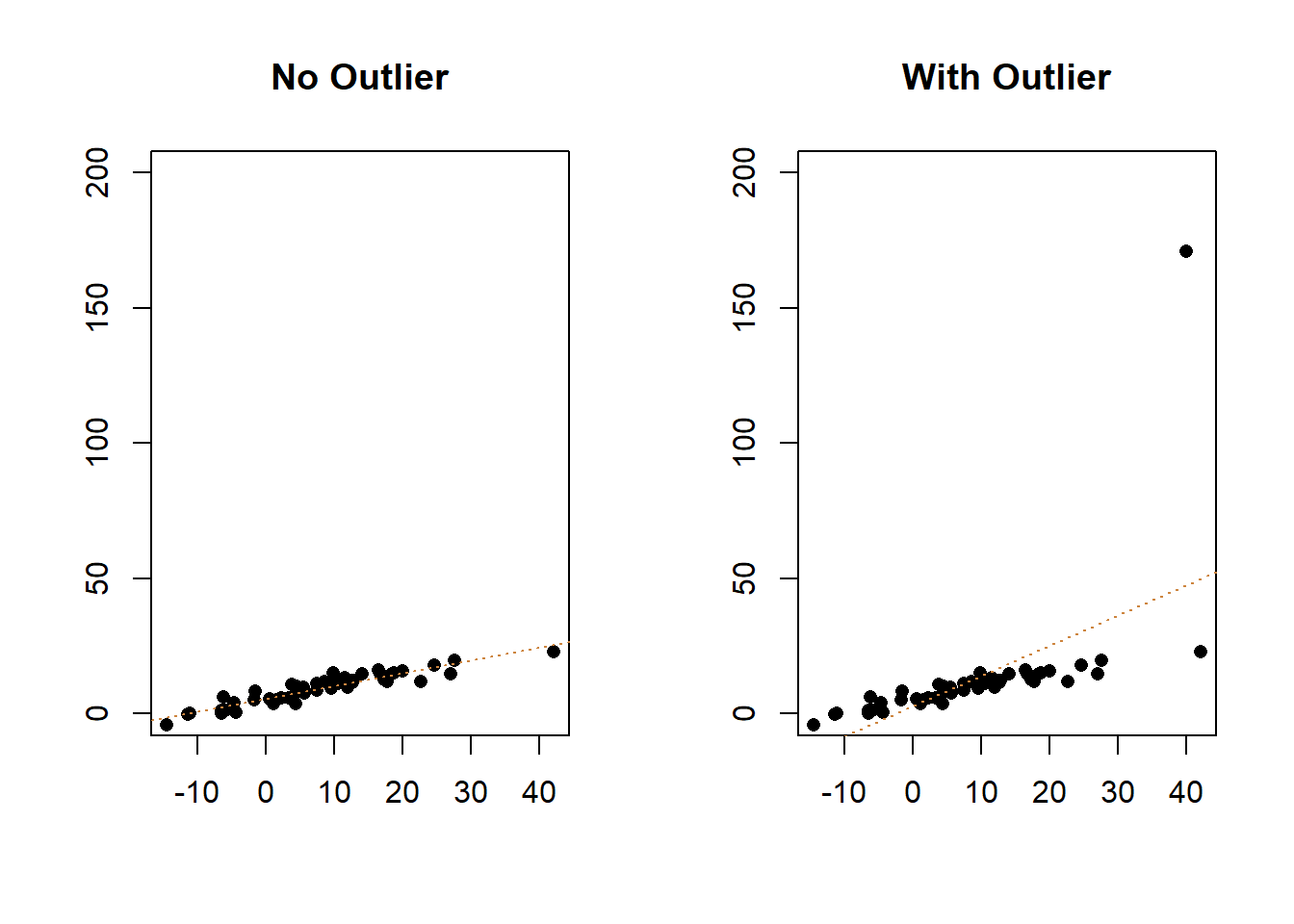
You can see above that the slope of the line of best fit has changed, shifting upwards to try and capture the information from that outlier. The line isn’t just a bad fit for the outlier, it’s also a worse fit for all of the data now. While the adjusted R-Squared for the original data was .8618, that drops to .3131 with the outlier.
So what can we do about an outlier? Not a lot. The important thing to do is look at your original data and make sure that the observation wasn’t generated by entry error. The y value for the outlier above is 171; was it supposed to be 17.1 maybe? If that’s the case correct the data and re-run the analysis. On the other hand, if the data is entered correctly, you probably should not remove the outlier. Yes, it makes your model look worse, and that bites. But if it’s a legitimate part of your data then it is part of the phenomenon that you’re trying to study.
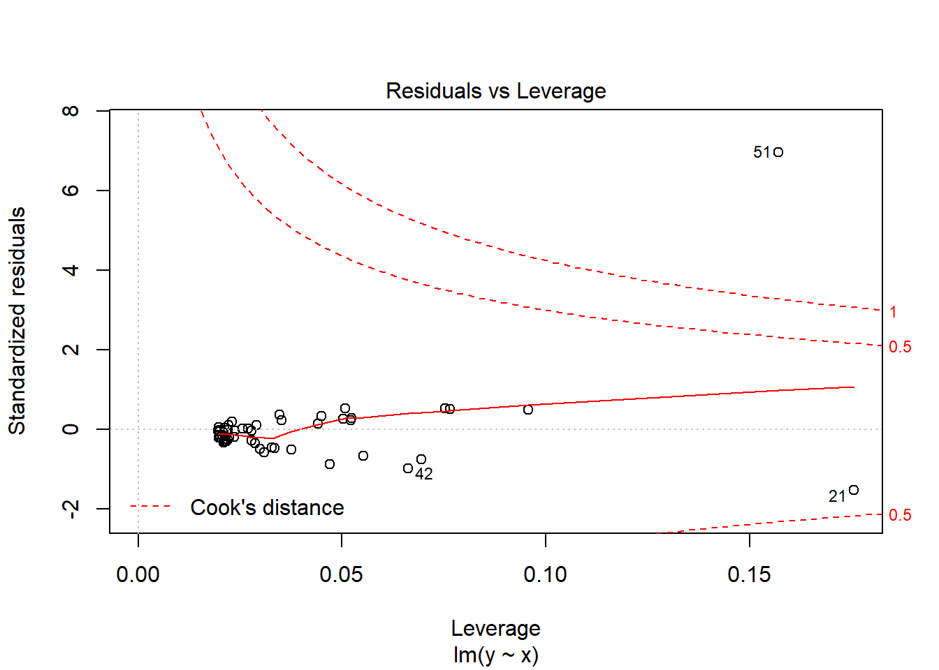
We can identify outliers in our regression using Cook’s Distance, which is a measure of the influence or leverage of a data point. What that means is, if we dropped each individual observation for our results, how big of a difference would that make to the results? An outlier, like the one above, significantly changed the model with its inclusion, so it has a lot of leverage on the model. Any value with a Cook’s D 3-times the mean is considered large. But again, those values are only really reviewed to see if there are any observations that should be reviewed for measurement error or validity.
The graph below displays the Cook’s distance for all the observations. What we care about there isn’t a pattern with the data in general, but rather whether any of our observations are above or below the red dashed line. The numbers identify the row number for any observations with high Cook’s distances, and we can see the 51st (the one we just added) has a lot of leverage.
16.1.9 The Importance of Theory
I want to leave you with some final thoughts about how to choose what to include in your regression before we do a round of practice. Developing models, and specifically figuring out what to include or exclude from your final regression, is one area where the social sciences are quite different from the data sciences or statisticians.
There are methods of allowing the model to essentially choose itself. You can set lots of variables to be tested in the model, and the model will run iteratively determining what is the least or most valuable variable to include. Essentially, statistics will tell you the point where you’ve included the combination of variables that best explain the variation in the dependent variable. That’s really valuable in some contexts. For instance, if you’re a company trying to figure out who is likely to buy your products, and you have data on a bunch of lifestyle and internet habits, it doesn’t matter to you which of those things are the best predictor. You just want to be able to identify your most-likely customers so that you can direct advertising to them.
In the social sciences, theory drives what independent variables you should include in your regression model. Whether the variable is significant or insignificant isn’t the largest concern, we don’t want to exclude a variable just because it fails to improve our model. If theory states that cities with greater population density should have higher crime rates, and you find that there’s no relationship between density and crime, that’s important! That’s a null finding, density hasn’t helped you to explain the variation in crime, but that’s theoretically relevant. In developing a regression model what you need to understand is what theory says should be important factors in predicting your dependent variable, and then include those variables. I can’t tell you here what will be theoretically relevant to whatever questions you’re going to ask, only you can understand that by reading the literature on the subject. See what other researchers have included in similar studies, and think about what should help you predict your outcome of interest.
16.2 Practice
That was a lot of information. Let’s work through it one more time from the top to the bottom to demonstrate how this might look in developing a regression model. This section will have the code visible.
We’re going to use a data set on student evaluations of professors. The dependent variable is the overall teaching evaluation score for a given class, on a scale of 1 (very unsatisfactory) to 5 (excellent).
TeachingRatings <- read.csv("https://raw.githubusercontent.com/ejvanholm/DataProjects/master/TeachingRatings.csv")
head(TeachingRatings)
## minority age gender credits beauty eval division native tenure
## 1 yes 36 female more 0.2899157 4.3 upper yes yes
## 2 no 59 male more -0.7377322 4.5 upper yes yes
## 3 no 51 male more -0.5719836 3.7 upper yes yes
## 4 no 40 female more -0.6779634 4.3 upper yes yes
## 5 no 31 female more 1.5097940 4.4 upper yes yes
## 6 no 62 male more 0.5885687 4.2 upper yes yes
## students allstudents prof
## 1 24 43 1
## 2 17 20 2
## 3 55 55 3
## 4 40 46 4
## 5 42 48 5
## 6 182 282 6We have a few independent variables to test.
- minority - Does the instructor belong to a minority (non-Caucasian)?
- age - the professor’s age. gender - indicating instructor’s gender. credits - factor. Is the course a single-credit elective (e.g., yoga, aerobics, dance)? beauty - rating of the instructor’s physical appearance by a panel of six students, averaged across the six panelists, shifted to have a mean of zero. division - Is the course an upper or lower division course? (Lower division courses are mainly large freshman and sophomore courses)? native - Is the instructor a native English speaker? tenure - Is the instructor on tenure track? students - number of students that participated in the evaluation. allstudents - number of students enrolled in the course. *prof - indicating instructor identifier.
We’ll drop prof, the unique identifier for each professor, but we’ll include all of the other variables. I think there’s an argument that any can have an interesting effect, and data sets that are built into R typically don’t contain extraneous data for no reason.
So let’s first look at our regression results below.
##
## Call:
## lm(formula = eval ~ minority + age + gender + credits + beauty +
##     division + native + tenure + students + allstudents, data = TeachingRatings)
##
## Residuals:
##      Min       1Q   Median       3Q      Max
## -1.90186 -0.30613  0.04462  0.36992  1.10919
##
## Coefficients:
##                Estimate Std. Error t value   Pr(>|t|)
## (Intercept)    3.801478   0.185771  20.463    < 2e-16 ***
## minorityyes   -0.165222   0.076515  -2.159   0.031350 *
## age           -0.002056   0.002677  -0.768   0.442817
## gendermale     0.203478   0.051443   3.955 0.00008869 ***
## creditssingle  0.560533   0.116680   4.804 0.00000212 ***
## beauty         0.145758   0.032194   4.527 0.00000765 ***
## divisionupper -0.044795   0.056792  -0.789   0.430664
## nativeyes      0.235691   0.106459   2.214   0.027332 *
## tenureyes     -0.051233   0.062578  -0.819   0.413384
## students       0.007427   0.002301   3.228   0.001338 **
## allstudents   -0.004627   0.001396  -3.313   0.000996 ***
## ---
## Signif. codes:  0 '***' 0.001 '**' 0.01 '*' 0.05 '.' 0.1 ' ' 1
##
## Residual standard error: 0.5087 on 452 degrees of freedom
## Multiple R-squared:  0.1776, Adjusted R-squared:  0.1594
## F-statistic: 9.764 on 10 and 452 DF,  p-value: 7.822e-15
We won’t go through the results of the regression line by line, I’m just going to pull out a few of the results. Interestingly, one of the reasons this data set exists is because they also got professors rated for their overall attractiveness. As predicted, a one unit increase in beauty rating is associated with an additional .145 points on the evaluations, holding all else constant, and that change is significant. In addition, were, females received lower evaluations, as did foreign-born and minority teachers. Larger classes in terms of the number of students were rated lower, while teachers in single credit elective courses got higher scores.
How did the model do overall? Well, the adjusted R-Squared was .1594. So, not awful… but not great. There’s still a substantial amount of the variation in evaluations that we aren’t able to explain with all those variables. In particular, we don’t have any measure of how good a teacher the teacher is. Now, that’s what the evaluation is supposed to be rating, but at the same time we observe that more attractive teachers are rated higher. We also don’t know the subject for any of the classes. Maybe knowing the grade distribution would be helpful too.
Back to the variables we have. Say we are deciding whether to include the variable tenure in our final model. We can run it with and without tenure, and compare the AIC for the two models. AIC() is a command that is available in base R ( so it doesn’t require a package). In order run it you need to save the lm() command as an object, like below. Make sure you don’t save the entire model summary, just the lm(). So we’ll first save a regression as reg_withtenure with all the variables, and a second one without tenure to see if that variable improves our model.
reg_withtenure <- lm(eval~minority + age + gender + credits + beauty + division + native + tenure + students + allstudents, data=TeachingRatings)
reg_notenure <- lm(eval~minority + age + gender + credits + beauty + division + native + students + allstudents, data=TeachingRatings)
AIC(reg_withtenure)
## [1] 700.941## [1] 699.6271The regression without tenure as an independent variable had a lower AIC, so we would be justified in removing it. however, if tenure is something we think should be important to predicting teaching evaluations, we should still include it and report the null result.
Does our regression violate any of the assumptions we described earlier? We can observe most of those just by graphing them. What I did earlier was save the regression results as the object ‘res’. You can graph regression results in R just by placing that object in the plot() command, as I do below. There are four traditional graphs shown for regression results. I use par(mfrow=c(2,2)) so that the graphs show in a 2 by 2 pattern so that they don’t take up too much space.
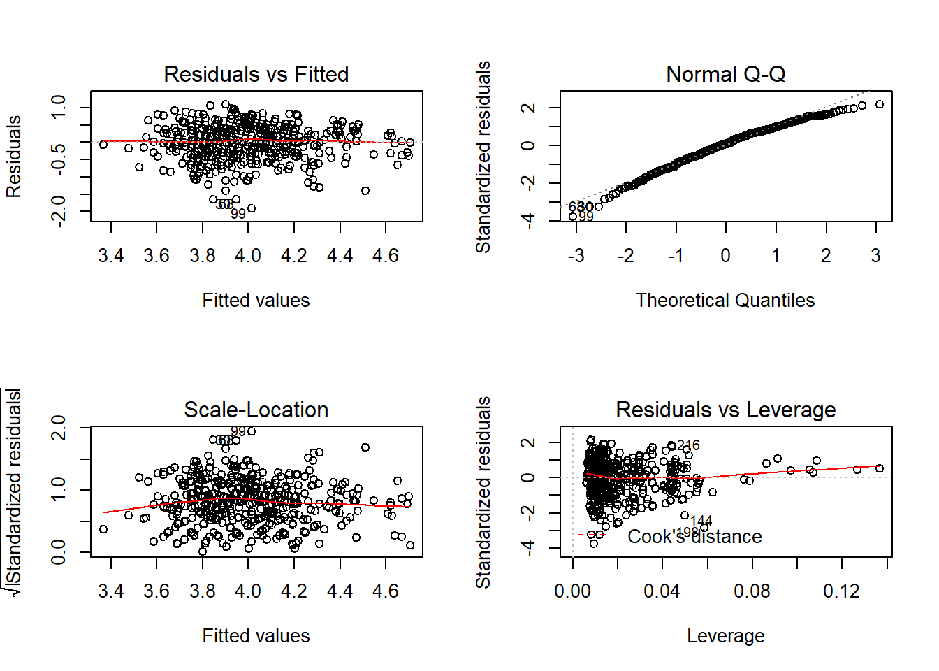
We produced some of those graphs above individually, let’s work through them one-by-one to make sure we’re getting what we learn from them. We’ll start at the top left and move clockwise.
Residuals vs Fitted in the upper left corner is used to checks whether a linear model is appropriate. The red horizontal is at y=0, to help highlight how evenly points are split above and below that point. At any predicted value in the data, the mean of the residuals should be zero, and we’d like to see that our residuals do not have any distinct pattern. This graph isn’t perfect, but that’s not expected, so this model would pass linearity.
Normal Q-Q, upper right, is used to examine whether the residuals are normally distributed. The points should follow the straight dashed line as closely as possible; it’s typically for there to be a little bit of a bend at the ends of the line, but nothing too distinct. The calculations required to create the plot vary depending on the implementation, but essentially the y-axis is the sorted data (observed, or sample quantiles), and the x-axis is the values we would expect if the data did come from a normal distribution (theoretical quantiles).
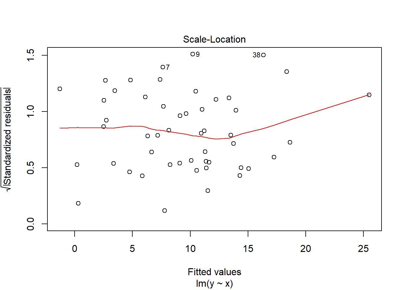
Scale-Location in the bottom left checks the homogeneity of variance in the residuals. What we want to see is that there is a horizontal line in the middle has points equally spread above and below it; if the line isn’t horizontal, that’s an indication that some part of your data is suffering from heteroscedasticity. A horizontal line is a good sign of homoscedasticity, which is what we want.
Residuals vs Leverage plot identifies influential cases that might influence the regression results when included or excluded from the analysis. Any rows that are identified by name in the plot are considered to have a lot of leverage and they’ll be placed outside the dashed red lines. Here, there are no points outside those lines, which means there aren’t any outliers. If there were, they would likely deserve additional scrutiny, but it is not recommended that you remove outliers.
Okay. So our model didn’t violate any assumptions. Finally, let’s see if there is any multicollinearity. We can test for multicollinearity using vif() from the car package.
##    minority         age      gender     credits      beauty    division
##    1.225254    1.196876    1.136262    1.237300    1.141156    1.280655
##      native    students allstudents
##    1.142814   19.135157   19.526222
We have some issues there. The number of students and the number of students that completed the evaluation are correlated. That makes sense, classes with more students are likely to have more evaluations submitted, even if a lower percentage do. One problem with those variables is that they’re probably measuring the same thing then (overall size of the class). We can make an adjustment then and replace the number of students that submitted evaluations with one that is the eprcentage of evalautions submitted for each class. That uses the unique infotmation that students is providing, while avoiding the collinierity.
TeachingRatings$evalpct <- TeachingRatings$students/TeachingRatings$allstudents
reg_notenure2 <- lm(eval~minority + age + gender + credits + beauty + division + native + evalpct + allstudents, data=TeachingRatings)
summary(reg_notenure2)
##
## Call:
## lm(formula = eval ~ minority + age + gender + credits + beauty +
## division + native + evalpct + allstudents, data = TeachingRatings)
##
## Residuals:
## Min 1Q Median 3Q Max
## -1.96013 -0.29767 0.04342 0.35082 1.29111
##
## Coefficients:
## Estimate Std. Error t value Pr(>|t|)
## (Intercept) 3.2108087 0.2096464 15.315 < 2e-16 ***
## minorityyes -0.2053037 0.0752776 -2.727 0.006634 **
## age -0.0013382 0.0026138 -0.512 0.608932
## gendermale 0.1890506 0.0503845 3.752 0.000198 ***
## creditssingle 0.5795145 0.1108772 5.227 0.000000264 ***
## beauty 0.1366760 0.0319002 4.284 0.000022384 ***
## divisionupper -0.0247056 0.0551717 -0.448 0.654516
## nativeyes 0.2292914 0.1048956 2.186 0.029334 *
## evalpct 0.7042906 0.1539113 4.576 0.000006130 ***
## allstudents 0.0002547 0.0003512 0.725 0.468626
## ---
## Signif. codes: 0 '***' 0.001 '**' 0.01 '*' 0.05 '.' 0.1 ' ' 1
##
## Residual standard error: 0.503 on 453 degrees of freedom
## Multiple R-squared: 0.1944, Adjusted R-squared: 0.1784
## F-statistic: 12.14 on 9 and 453 DF, p-value: < 2.2e-16## [1] 689.423## minority age gender credits beauty division
## 1.235526 1.199069 1.132739 1.235669 1.155962 1.248594
## native evalpct allstudents
## 1.144272 1.214753 1.269450Cool. The AIC is improved (smaller), and there is no multicollinierity left in the model. I’ll judge this model good to go for the moment.