9 Introduction to R
You’ve made it this far. In theory you know how to collect your data now. You might have done that by conducting interviews or running a survey, or just by visiting an archive like the General Social Survey website. Having data is worth something, but it’s not worth everything. You have to do something with the data in order to answer any questions with it.
The rest of this book is focused on that goal - using the data you collected in order to answer the questions you want to be able to ask. A lot of the time we use statistics to answer those questions, at least partially. Sometimes we’ll use the basic calculations you probably did in a high school stats class and sometimes using something more complicated. Statistics is a substantial part of how social scientists know anything about the world. But this book wont focus on how to calculate a standard deviation by hand, because you don’t have to. It’s good for understanding what the measure means, but software can do that work for you lightning fast - the more important skill is knowing what to do with it once it is calculated.
The next set of chapters will all be structured the same way. The first half of the chapter will introduce a topic (in this chapter R and programming) and the second half will focus on examples and practice. You can read the first half without being concerned about the second half, and you can just go practice the second half if you already know everything you need to about the topic.
The second half of the chapter will generally repeat the material in two forms. I’ll describe all the steps involved in whatever we’re learning, and I’ll walk you through those steps using videos too. That gives you a few opportunities to see the material. If you get stuck practicing it’ll be frustrating. I still get frustrated pretty often when coding. What I would recommend is slowing down, looking back at what you did and just trying to reproduce exactly what is in the book as closely as possible.
9.1 Concepts
9.1.1 What is R
R is a programming language and environment for data analysis that is popular with researchers from many disciplines. R refers both to the computer program one runs, as well as the language one uses to alter data within the environment. R only speaks R, and so like traveling to a foreign country it is useful to learn the local language in order to communicate. You call yell at R in English as long as you want, but it can’t produce your data unless you ask correctly. Fortunately, R’s language is based on English and it wants to be as straightforward as possible
9.1.2 Why Use R?
There are other statistical packages that similar research methods classes use, including Stata and SPSS. One of the greatest benefits of R is the price: free. Access to Stata for a one semester class costs $45-125, and extended access costs more. And like Apple they update the software periodically, which means purchasing a new license. R is an open source software that anyone can use free of charge forever. That means whatever skills you learn you can continue to develop after the class ends.
Many people have access to Excel as a spreadsheet program through Microsoft Office, but R is faster and more flexible for data analysis. Excel is a drag-and-drop program that does not produce reproducible analysis. R, as a programming language, allows users to create a ‘script’ that the computer runs in order to output analysis. That means the script can be reusable, shareable, and iterative, which will have significant benefits if you continue with data analysis after the class. Luckily, R is a relatively straightforward introduction to programming.
Me justifying that you should learn to code because it will benefit you after the class and you can write something called a script probably sounds weird though. The majority of readers wont be interested in doing anything related to this class after the semester, and you have no idea what a script or reproducible analysis is. Using Excel would be more user friendly - there would be no language to learn, and the data you’re using is always right in front of you. I’ve done that before in a similar class, and actually using Excel as a tool is just as a difficult for beginners, and the ceiling on how useful it can be for working with data is considerably lower. Take this class as an opportunity and gentle introduction to a really valuable career skill: programming.
9.1.3 Why learn to program?
Data analytics is a quickly growing field with numerous job possibilities. The skills you learn in this class, if more fully developed, can be applicable to any industry, from Google to banks to government to a lemonade stand.
Computer programming is a flexible skill that can help you to manage laborious processes. It can stimulate creative thinking, grow your problem solving capabilities, and can help teach persistence. All of that with a valuable on the job market.
Data Scientist has been called the sexiest job of the 21st Century.
If you wont take my word for it, President Obama once stated that every kid should learn how to code/program.
Let’s give it a shot in this class, and see if it’s a skill you’d like to continue developing.
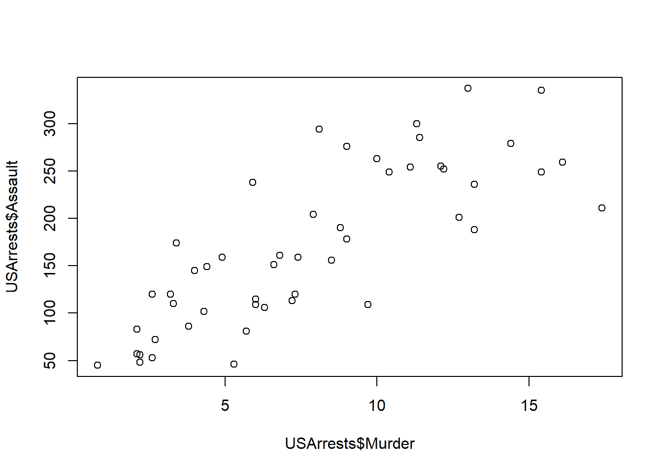
I’ll make one final argument in favor of coding. It’s a bit like doing magic of casting spells. You get to speak an arcane language that not everyone understands and when you do speak it things happen. If I write a statement like “a graph that shows the relationship between murder and assault rates for US states” the sentence does nothing. It just sits there, and you can read that sentence, but nothing happens. If I write a spell though like plot(USArrests$Murder, USArrests$Assault) suddenly it transforms into what I want.
Do you remember the movie the Sorcerer’s Apprentice? Mickey could have mopped the floor on his own, but that would be tedious. Instead he used magic to do it and because of that magic he was able to do hundreds of hours of manual work with the wave of a wand.
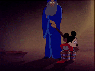


Unfortunately, that went badly in the movie. We have to be careful while coding or casting spells because having something get mistranslated might have unintended consequences. But it’s a more efficient way to use data and with a little practice you might amaze yourself with the things you can create.
9.2 Downloading R
9.2.1 The R Programming environment
R can be downloaded from the r-project.org
There is a link on the left. You’ll need to select a ‘mirror’ to download from. Don’t worry too much about that, the code for R is housed at multiple locations around the world so that it’s always available even if one site gets knocked off line. Generally, you should download from the location that is closest to you, but I have never noticed a difference. For New Orleans, that’s either Oak Ridge, Tennessee or Dallas, Texas. Click the link and follow the directions for installing the program.
9.2.2 R studio
The R package you just downloaded can fully operate on its own, but we want to download a second program (an additional integrated development environment) in order to make using R a little more straight forward. R Studio uses the R language while organizing our data sets, scripts, and outputs in a more user-friendly format. Luckily, it’s free too and can be downloaded from rstudio.com. Click the link for R studio Desktop and follow the prompts to install.
Note: in order for R Studio to operate R must also be loaded on the computer too. R can operate on its own, and you’re welcome to use it, but class examples will be shown using R Studio.
The following will walk you through all of those steps again.
9.2.3 Getting started in R studio
Let’s open R Studio and see what we have downloaded.
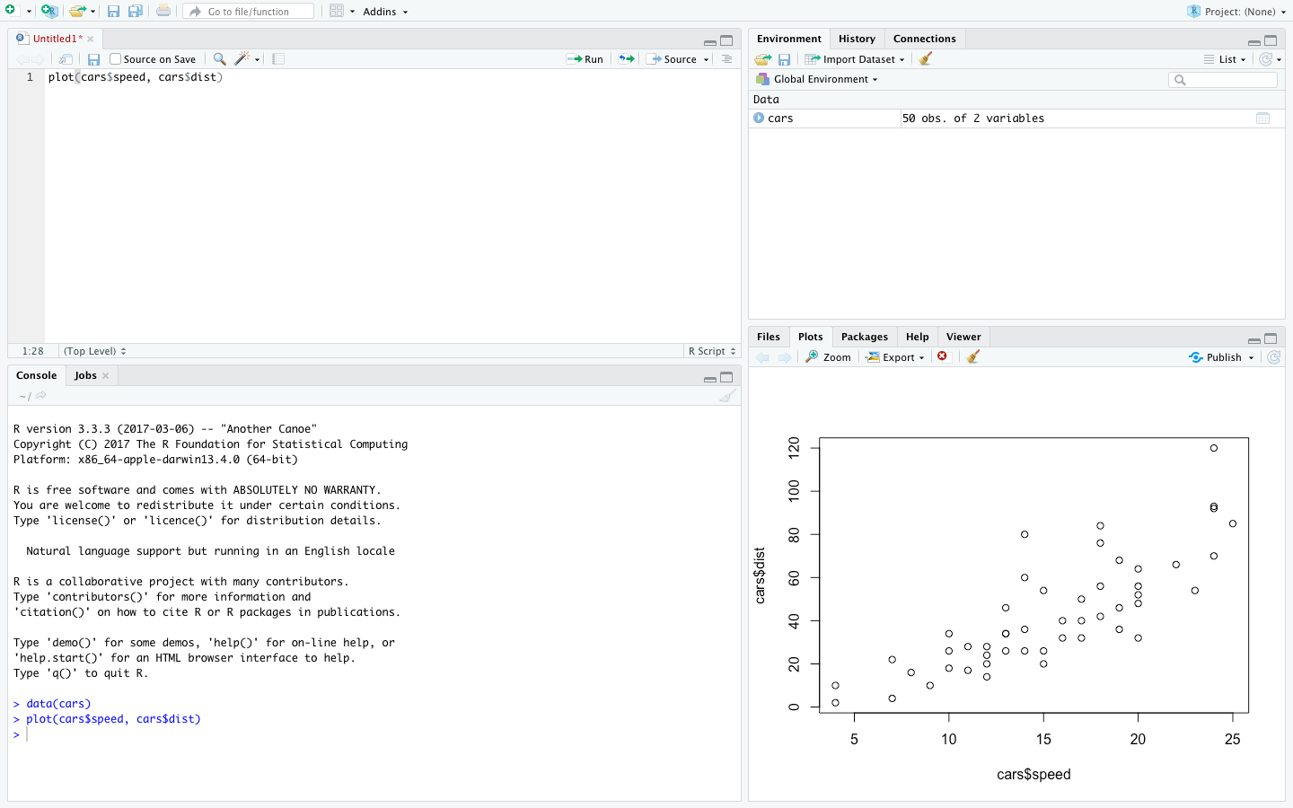
The program opens with 3 sections (or boxes) displayed, although there are four. If you click the small green button in the upper left, you can create several types of documents in R. Let’s open a script, which should now add our fourth section.
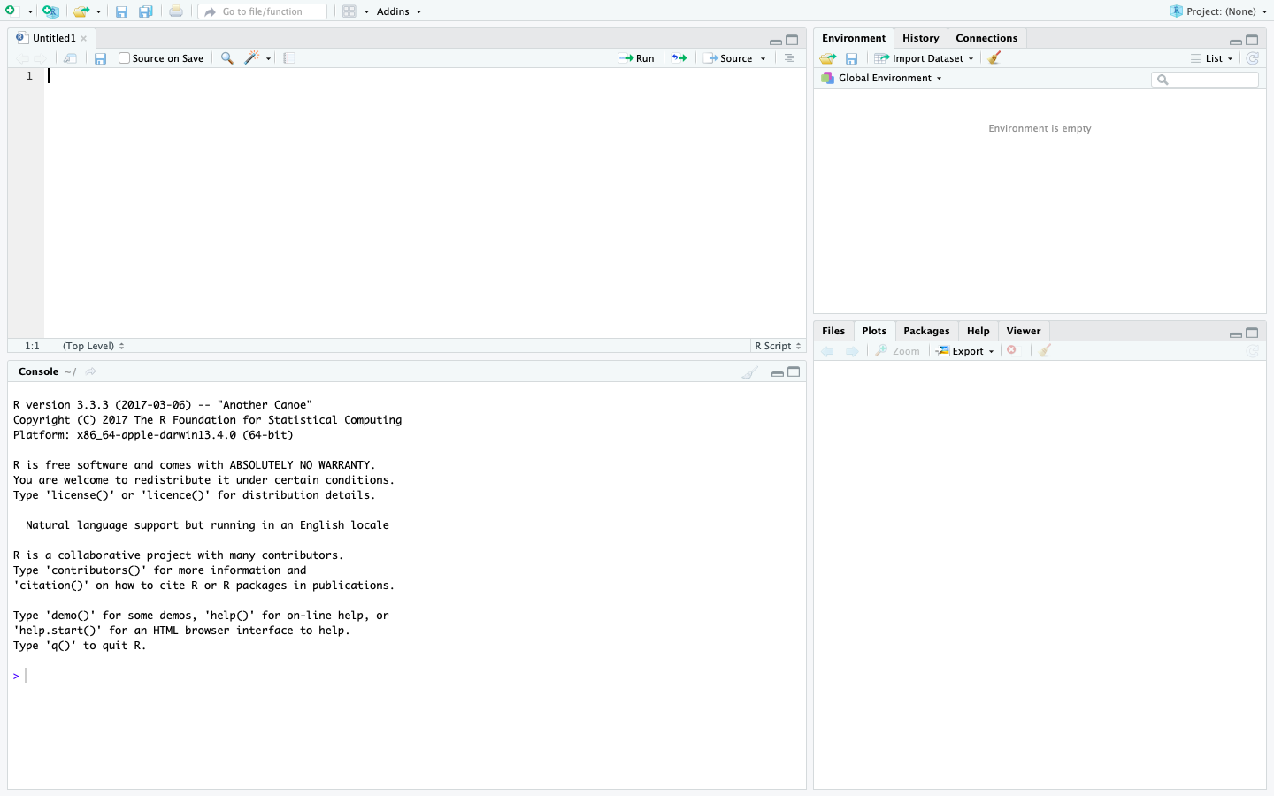
The upper left quadrant is called the script, which is where we can write out codes to be executed. You can enter the code without writing it out first, but by writing in the script we can be preserve and reuse it. If you’re going to use a line of code multiple times, it’s good to have it written because then you can re-execute it without re-writing it. Because scripts can get up into thousands of lines, it’s good to have everything written out so that it can be reviewed and checked. These are like the directions for a recipe we used in baking our data.
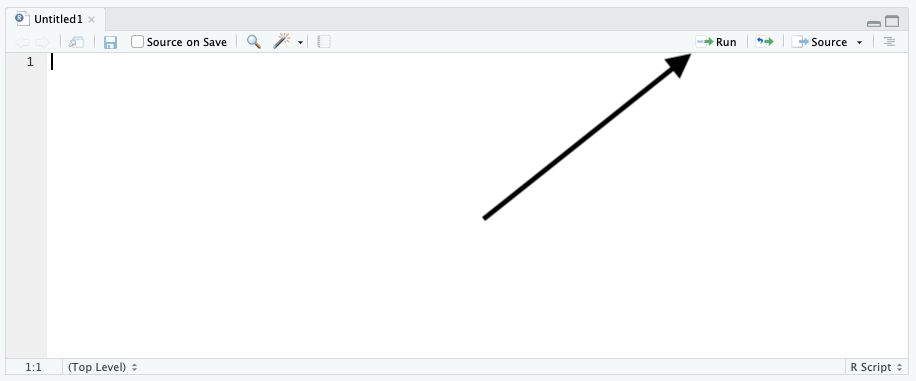
In order to execute code that you write in the script, you need to press the ‘run’ button in the upper-center of R studio. That’ll send the code to be executed and provide output below.
The bottom left is called the output. If you write the command 2+5 in your script and run it, that line of code and the result will appear in the output: 7. Any code you run will display itself processing in that section, and any statistics you produce will come at the end (like the answer to 2+5).
The upper right is called the environment, which is where data you have available to you in R will appear. You won’t see the data itself, but the environment gives you a record of everything that is available in R Studio for you at that moment. If you do want to see the actually data you have saved, you can type View() with the name of the data set.
The bottom right section actually has a few different uses, but we can concentrate now on the graphical output. If we produce a plot or graph of our data, that is where it will appear once the data has executed.
The picture below shows all 4 sections in use. You can see the brief script I wrote, the output of that script, the data I’m using (cars) and the graph I’ve created.
You can see those four sections described again below in this video.
9.3 Practice
So that’s an introduction to R Studio, and now you hopefully have it installed on your computer and have it open. They say that practice makes perfect, and that’s just as true with coding as anything else. No one is born knowing how to code. Its one of the best example I’ve seen of Malcolm Gladwell’s 10,000 hours, where the only way to get good is to keep trying. We’re almost at the end of your first hour (assuming you watched both those videos all the way through).
What we describe in this chapter wont be exciting. We can’t jump right into the type of coding that is going to instantly give you answers to researcher questions like what makes people happy, but these are the basic building blocks necessary to answer those questions. We’re at the point in learning a new language when we’re practicing words like “blue” and “shirt” and “I am”. One week of Spanish class doesn’t make you fluent, and this chapter wont make you a data scientist. But it is a necessary first step.
Let’s quickly review some of the things we can do in R that are most useful. I would recommend creating a new script (hint: top left corner) in R Studio and entering and running these commands as they are outlined. That applies to future chapters as well. As I run each command in the textbook you’ll both see the code that I ran and the output.
This chapter essentially describes in writing the contents of a video that is at the end of the chapter. You can use either source to learn the material, or both. However you prefer to learn, seeing it more directly demonstrated or reading the steps, the choice is yours. My goal is to provide as many resources as I can.
Reading a description of operations is a good start, but much of coding is muscle memory and takes practice at the syntax and structure of commands. As you enter the commands, try to tweak them and break them. Figure out what’s optional in what I’m writing and what’s necessary.
There is a tradition that you should first introduce yourself by saying “hello world”. In R, you can do that by writing it directly into the script and executing (clicking on the run button.
## [1] "hello world!"Or you can save it by giving it a name. When you save something you create or read data into R it creates an object, which will appear under the environment on the top right of the screen.
## [1] "hello world!"When you try to execute each command by hitting run, make sure that you’ve highlighted all of the code you want to enter. You can run thousands of line of code at any given time just by highlighting it. But unless you tell R that is the line of code you want to run, it wont do anything.
Let’s take a second to really break down both lines of code we just ran.
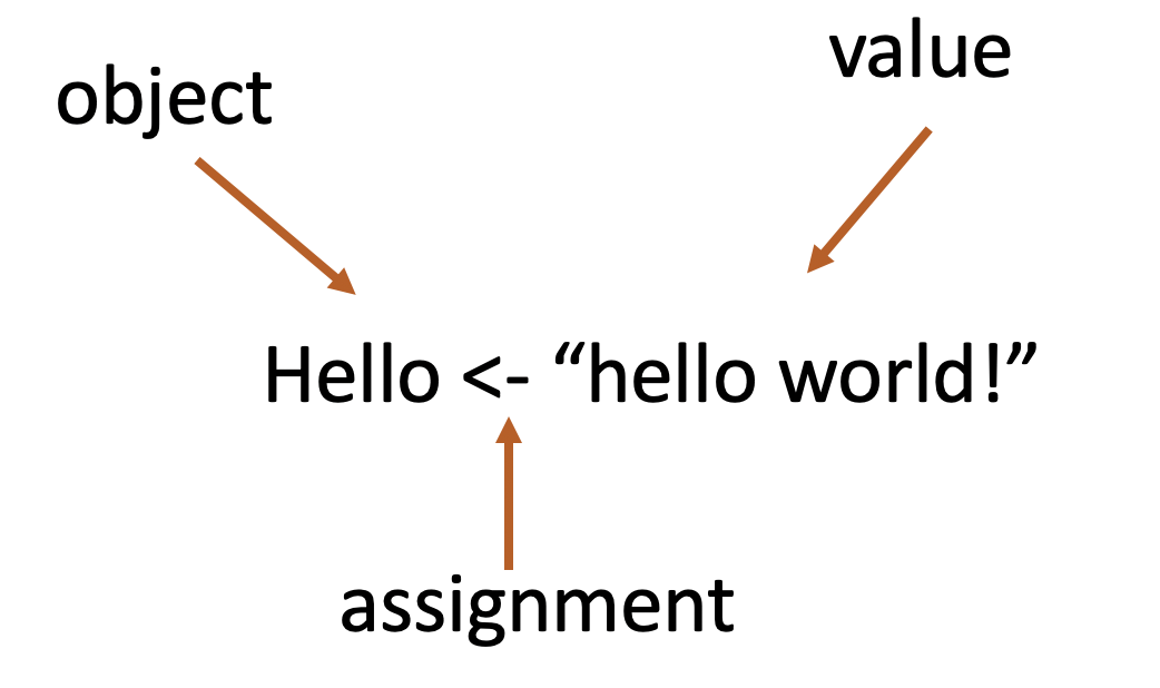
In the first one we’re saving or assigning the value “hello world!”. Each part of that code is playing a part, there’s nothing wasted when we’re writing code. hello is going to become an object, that’s what we’re creating with the line of code. The arrow (<-) tells R what we’re assigning to the “hello”. And the right side of the arrow is the value we’re creating. We can’t flip around the arrow, we can’t save values from the left side of an arrow to the right side, we’ll always use the same structure of working from left to right.
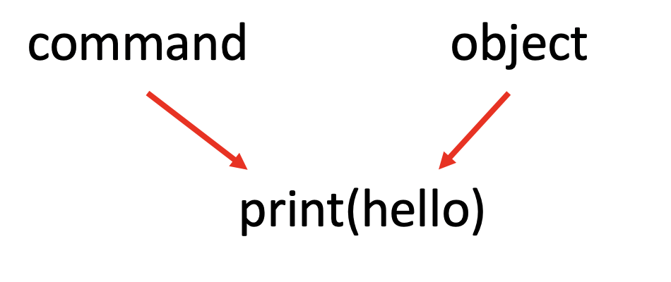
Each line of code generally includes a command, which is something you can tell R to do. For instance, print() is a command. R has it built into its system what to do if you tell it print(). But you also have to tell it what to do that to - what do you want to print? What you want to print is the object, in this case hello. You use a command to do an action to an object. You can think of commands as verbs and objects as nouns. Timmy runs. Print hello. runs(Timmy). print(hello).
We can also save numbers or anything else as an object in R. For instance, we can create an object named x and give it the value of 2.
## [1] 2Or we can create an object y with multiple values. We can store lists as an object by placing c in front of parentheses. the letter ‘c’ stands for concatenate or combine.
## [1] 1 2 3We can use R as a calculator by entering math equations:
## [1] 5The reason to create objects is because we can then use them later without having to reenter their components. For instance we can multiply x by y using the values we supplied earlier.
## [1] 2 4 6That’s sort of a brief introduction to creating data in R, the goal of this class isn’t to have you entering numbers line by line into .The whole benefit of using R is that it can work with entire data sets really efficiently. So let’s jump forward and talk about how to read data that we have external of R into R.
R actually comes with a lot of data sets built into it’s software. We’ll sometimes use those data to create examples. You can see the data that is present in R by writing data(). You can call one of those data sets out of the background into being used by writing data() with the name of the desired data set inside.
## Murder Assault UrbanPop Rape
## Alabama 13.2 236 58 21.2
## Alaska 10.0 263 48 44.5
## Arizona 8.1 294 80 31.0
## Arkansas 8.8 190 50 19.5
## California 9.0 276 91 40.6
## Colorado 7.9 204 78 38.7
## Connecticut 3.3 110 77 11.1
## Delaware 5.9 238 72 15.8
## Florida 15.4 335 80 31.9
## Georgia 17.4 211 60 25.8
## Hawaii 5.3 46 83 20.2
## Idaho 2.6 120 54 14.2
## Illinois 10.4 249 83 24.0
## Indiana 7.2 113 65 21.0
## Iowa 2.2 56 57 11.3
## Kansas 6.0 115 66 18.0
## Kentucky 9.7 109 52 16.3
## Louisiana 15.4 249 66 22.2
## Maine 2.1 83 51 7.8
## Maryland 11.3 300 67 27.8
## Massachusetts 4.4 149 85 16.3
## Michigan 12.1 255 74 35.1
## Minnesota 2.7 72 66 14.9
## Mississippi 16.1 259 44 17.1
## Missouri 9.0 178 70 28.2
## Montana 6.0 109 53 16.4
## Nebraska 4.3 102 62 16.5
## Nevada 12.2 252 81 46.0
## New Hampshire 2.1 57 56 9.5
## New Jersey 7.4 159 89 18.8
## New Mexico 11.4 285 70 32.1
## New York 11.1 254 86 26.1
## North Carolina 13.0 337 45 16.1
## North Dakota 0.8 45 44 7.3
## Ohio 7.3 120 75 21.4
## Oklahoma 6.6 151 68 20.0
## Oregon 4.9 159 67 29.3
## Pennsylvania 6.3 106 72 14.9
## Rhode Island 3.4 174 87 8.3
## South Carolina 14.4 279 48 22.5
## South Dakota 3.8 86 45 12.8
## Tennessee 13.2 188 59 26.9
## Texas 12.7 201 80 25.5
## Utah 3.2 120 80 22.9
## Vermont 2.2 48 32 11.2
## Virginia 8.5 156 63 20.7
## Washington 4.0 145 73 26.2
## West Virginia 5.7 81 39 9.3
## Wisconsin 2.6 53 66 10.8
## Wyoming 6.8 161 60 15.6We can view all of the data by writing View() and the name of the data set. View() is a command in R. It’s telling R what I want it to do, but I have to tell it what to do it to. I already have multiple objects loaded into R, specifically x and y and USArrests. I don’t want to see them all, I just want to see USArrests, so I have to enter that name into the command View(USA)
Not all data is built into R though. In fact, most of the data you’ll want to use in the real world isn’t already built in - the stuff R contains is really only useful for examples and basic practice. I’ll cover how to read in data from your computer in a later chapter, everything you need to run the examples in this book is saved online in an open directory on Github. Github is a free and open source website where people can share data. I post the data you’ll need there to make it easy to access. You can see all of the data that is currently available by following this link: https://github.com/ejvanholm/DataProjects
You can read in one of those data sets with the command read.csv() and the web link to the raw data.
We can also see the top few lines of a data set using head(), with the general default being to show 5 or 6 lines of the data. I can also see the bottom using tail()
## X district school county grades students
## 1 1 75119 Sunol Glen Unified Alameda KK-08 195
## 2 2 61499 Manzanita Elementary Butte KK-08 240
## 3 3 61549 Thermalito Union Elementary Butte KK-08 1550
## 4 4 61457 Golden Feather Union Elementary Butte KK-08 243
## 5 5 61523 Palermo Union Elementary Butte KK-08 1335
## 6 6 62042 Burrel Union Elementary Fresno KK-08 137
## teachers calworks lunch computer expenditure income english read
## 1 10.90 0.5102 2.0408 67 6384.911 22.690001 0.000000 691.6
## 2 11.15 15.4167 47.9167 101 5099.381 9.824000 4.583333 660.5
## 3 82.90 55.0323 76.3226 169 5501.955 8.978000 30.000002 636.3
## 4 14.00 36.4754 77.0492 85 7101.831 8.978000 0.000000 651.9
## 5 71.50 33.1086 78.4270 171 5235.988 9.080333 13.857677 641.8
## 6 6.40 12.3188 86.9565 25 5580.147 10.415000 12.408759 605.7
## math
## 1 690.0
## 2 661.9
## 3 650.9
## 4 643.5
## 5 639.9
## 6 605.4## X district school county grades students
## 415 415 69682 Saratoga Union Elementary Santa Clara KK-08 2341
## 416 416 68957 Las Lomitas Elementary San Mateo KK-08 984
## 417 417 69518 Los Altos Elementary Santa Clara KK-08 3724
## 418 418 72611 Somis Union Elementary Ventura KK-08 441
## 419 419 72744 Plumas Elementary Yuba KK-08 101
## 420 420 72751 Wheatland Elementary Yuba KK-08 1778
## teachers calworks lunch computer expenditure income english
## 415 124.09 0.1709 0.5980 286 5392.639 40.40200 2.050406
## 416 59.73 0.1016 3.5569 195 7290.339 28.71700 5.995935
## 417 208.48 1.0741 1.5038 721 5741.463 41.73411 4.726101
## 418 20.15 3.5635 37.1938 45 4402.832 23.73300 24.263039
## 419 5.00 11.8812 59.4059 14 4776.336 9.95200 2.970297
## 420 93.40 6.9235 47.5712 313 5993.393 12.50200 5.005624
## read math
## 415 698.9 701.7
## 416 700.9 707.7
## 417 704.0 709.5
## 418 648.3 641.7
## 419 667.9 676.5
## 420 660.5 651.0When you’re first learning to write code it’s useful to write it in an R script, as I’ve demonstrated above. That gives you the opportunity to practice and re-write your code, and copy what you did earlier for later projects. I often recycle code, borrowing it from one project to the next where it’s necessary. Coding very much follows the adage that ‘the only rule is that it has to work’. There aren’t awards for writing the most new code, just that the code you use works. Steal from yourself. Look on the internet and find code that can answer your problems. Coding is all about getting the most output for the least work.
9.3.1 Getting Help
One of my favorite things about R is how much information there is online to help someone with problems. If you feel stuck, googling “introduction to R Studio” will produce thousands of links, and if you want to search “how to create a plot in R” you’ll find lots of help from a really engaged community. If this is your first time opening R it’s probably overwhelming, but the best way to move forward is to practice. As the semester goes we will get more comfortable.
I hardly make it through a project without searching for an answer to something. And there are some commands I just haven’t memorized. There are a few on post-it notes stuck around my computer screen, and there are others I have to search every few weeks (“how to remove duplicate results”). The goal of learning R isn’t to immediately memorize every command, it’s to know what’s possible in R. And as you get more comfortable, more will become possible.
A few things that will probably trip you up. R is finicky about spelling and capitalization. It only knows how to do things if you spell them exactly right. It’s not going to interpret what you say if you forget a letter in the command. When you get error messages, and you will, read the command you wrote closely. The error message probably wont make sense to you, but it’s trying to tell you that it doesn’t understand what you want it to do.
Here is all of the code we executed in this chapter.
"hello world!"
hello <- "hello world!"
print(hello)
x <- 2
print(x)
y <- c(1, 2, 3)
print(y)
2*3
x * y
data()
data("USArrests")
View(USArrests)
CASchools <- read.csv("https://raw.githubusercontent.com/ejvanholm/DataProjects/master/CASchools.csv")
View(CASchools)
head(CASchools)
tail(CASchools)
names(CASchools)