Chapter 5 Creating Variables
This section focuses on the creation of new variables for your analysis as part of an overall strategy of cleaning your data. Often times, data will come to you coded in a certain way, but you want to transform it to make it easier to work with. Our analyses often focus on linear changes in a given variable, but data is typically not coded in such a way to represent those types of differences. We’ll explore that more below.
Some of the tools we need to practice with aren’t directly related to creating new variables or cleaning the data we have, but just understanding what issues there might be. Before you start analysis it’s necessary to step back and observe your data. Understand how the different values are coded and what you might need to do. So, each step below both focuses on figuring out what to do with our data, as well as doing it.
We’ll use the same file I was using in the earlier chapter on loading data, but we’ll load it in from GitHub so that it’s straightforward for anyone to access and use. Notice that we’re using the same read.csv() command, because that is how the file is saved even thought it’s located on the interwebs.
5.1 Using ifelse
We’ll save the file as a new object called ‘dat’ and start by taking a look at the top few lines with head() to get a feel for whats in the data.
dat <- read.csv("https://raw.githubusercontent.com/ejvanholm/DataProjects/master/RClass/cps_00003.csv")
head(dat)
## YEAR SERIAL MONTH HWTFINL CPSID REGION STATEFIP METRO METAREA
## 1 2018 1 11 1703.832 2.01708e+13 32 1 2 3440
## 2 2018 1 11 1703.832 2.01708e+13 32 1 2 3440
## 3 2018 3 11 1957.313 2.01809e+13 32 1 2 5240
## 4 2018 4 11 1687.784 2.01710e+13 32 1 2 5240
## 5 2018 4 11 1687.784 2.01710e+13 32 1 2 5240
## 6 2018 4 11 1687.784 2.01710e+13 32 1 2 5240
## STATECENSUS FAMINC PERNUM WTFINL CPSIDP AGE SEX RACE EMPSTAT
## 1 63 830 1 1703.832 2.01708e+13 26 2 100 10
## 2 63 830 2 1845.094 2.01708e+13 26 1 100 10
## 3 63 100 1 1957.313 2.01809e+13 48 2 200 21
## 4 63 820 1 1687.784 2.01710e+13 53 2 200 10
## 5 63 820 2 2780.421 2.01710e+13 16 1 200 10
## 6 63 820 3 2780.421 2.01710e+13 16 1 200 10
## LABFORCE EDUC VOTED VOREG
## 1 2 111 98 98
## 2 2 123 98 98
## 3 2 73 2 99
## 4 2 81 2 99
## 5 2 50 99 99
## 6 2 50 99 99The first few columns are what could be called administrative. They’re unique identifiers for the different observations, the timing of the survey they’ve taken, and a bit of other information. So for now we don’t need to pay much attention to MONTH, HWTFINL, CPSID, PERNUM, WTFINL, or CPSIDP.
The next few columns are concerned with different geographies we have for the observations. This data is for individuals, but we also know the individuals region (REGION), state (STATEFIP and STATECENSUS), and metropolitan area (METRO and METAREA). We’ll talk about those more in a later chapter on AGGREGATION, but we don’t need to worry about them at the moment.
So let’s start looking by looking at AGE. Age is the rare variable that typically comes “finished” for us. Sometimes, we don’t need to make any changes to get it ready for analysis.
## [1] TRUEWe can use the command is.numeric() to check whether the column AGE is numeric, and TRUE tells us that is correct. Age is numeric, which is what we would expect. We can check the summary statistics for it just to make sure everything looks as we expect.
##    Min. 1st Qu.  Median    Mean 3rd Qu.    Max.
##    0.00   20.00   40.00   40.17   59.00   85.00
That looks right to me. So AGE is ready to go if we want to use it as a numeric variable. We’ll talk more later about what we can do if we want to look at people based on their generations or categories of their age, rather than just using the years they’ve been alive as a variable.
What about the variable SEX? Let’s see what values we have in the column using the table() command. Table gives us a count of how many observations of each type we have.
##
##     1     2
## 59838 62906
Okay, so we have 1’s and 2’s. One issue is that we don’t know what those mean. We have more 2’s than 1’s, but we don’t know whether Male’s were coded as 1’s or 2’s so these values have no meaning to us at the moment. We need to look at the code book for the data to understand what those values represent about respondents. It’s really useful to look through the code book before you start using your data, because most of the questions we’re asking in this section could be answered by just reading it… but reading instructions is boring, so I usually skip it as long as I can. What does the code book tell us about the variable SEX?
1’s are Male and 2’s are Female. We can leave the variable as is and remember those values, or we can also create a new variable that’s named either Male or Female so that we know the gender of respondents a little more easily. To do that we can use the command ifelse().
##
##     0     1
## 62906 59838
Great, now anyone that was coded as a 1 in the column SEX is now coded as a 1 in the column Male. That isn’t a huge change, but now we can more intuitively know the gender of respondents by just looking at the column Male. We could also create a variable called Female for respondents that were 2’s for SEX.
##
##     0     1
## 59838 62906
It really doesn’t matter whether we create a column called Male or Female. They have the same information, just coded a little differently. And we wouldn’t need to create both, since if we have 1 we know everything the second variable tells us.
We’re going to use ifelse() statements a lot to get the data into the exact structure we want, so let’s take a closer look at it.
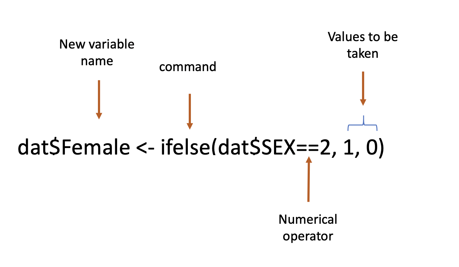
An ifelse statement reads a bit like a sentence. We’re asking R to determine which of two things is true, either the variable SEX equals 2 or it doesn’t. If it does equal 2 (dat$SEX==2), then we want the new variable we’re creating named Female to take the value 1 (the first of two options we’re giving). If the column SEX doesn’t equal 2, then the new variable should take the value 0. As a result, our new variable Female is a series of 0’s and 1’s.
An ifelse command has 3 essential parts. 1. What should it to see if it is true, 2. what should it do if that is true, 3. What should it do if that isn’t true. We need to supply the command with something to check, and two things to do depending on whether that is true or not.
The numerical operator in an ifelse statement is really important. Here we wanted to determine if the value of SEX was 2. We can use any numerical operator though. The table below displays common numerical operators and what they’re asking about for different variables. I’ll demonstrate more of these below.
| Numerical Operator | Effect |
|---|---|
| == | Equals |
| != | Doesn’t Equal |
| > | Greater than |
| >= | Greater or equal to |
| < | Less than |
| <= | Lesser or equal to |
So we used two examples of equals above. Let’s see how ‘doesn’t equal’ (!=) works out.
##
##     0     1
## 59838 62906##
## 0 1
## 59838 62906Exactly the same. We can either ask R to code all of the observations that are 2’s, or all of the observations that aren’t 1’s and we get the same essential result.
We can also use the greater than/lesser than with SEX because it’s a numerical variable.
##
##     0     1
## 59838 62906##
## 0 1
## 62906 59838If the values is equal to or less than 2 we coded the observation as a 1 in Female above, or we could code the observations that are equal to or less than 1 as 1 if the variable is Male. That’s a little more silly though since we only have two observations. Above we’ve been practicing creating dichotomous or dummy variables, which are variables which take two values. Either the new variable is a 1 or a 0 depending on the value of something else. We can also create categorical variables with words as our new values. Below we’re going to ask whether the column SEX is equal to 1, and if so make the new variable take the value “Male”, and otherwise give it the value “Female”.
##
## Female Male
## 62906 59838If our original data was coded as words, we can use the equal to operator to create new variables as well.
##
##     0     1
## 62906 59838And round and round we go. If the data is coded as words, we can only use the equal to/not qual to operator, because it wouldn’t make sense to be “greater than” a word like male or blue or fish. You’ll also need to be really careful with spelling. R will only code a value as 1 if the values in the column match what you write exactly.
Below I’m going to make a small typo and write “Mal” instead of “Male”. What do you think is going to happen?
##
##      0
## 122744
All of the observations are coded as 0. Why? I asked R to code anything that had the value “Mal” as a 1. Being that nothing in the column Gender is coded “Mal” everything is coded as 0. That’s why it’s important to be careful checking the values that your column has before using ifelse and to see the values your new variable has afterwards.
5.2 Lesser and Greater Than
Let’s go back to AGE to better show the utility of the “greater than” and “lesser than” operators". Let’s say we want to create a variable that takes the value of 1 if the person is over the age of 65. We’re not interested in just linear changes in Age as a person gets older, we’re intereted in differences between generations maybe.
##
##      0      1
## 100509  22235
It looks like 22235 respondents were over that age. What if we wanted to create a variable that takes the value of 1 if they’re under the age of 18?
##
##     0     1
## 94137 28607
We can also use multiple numerical operators in the same ifelse. Let’s say we want to create a variable that specifies if a person is a millennial. Millennials were born between 1981 and 1996, so for a survey from 2018 they would be between the ages of 22 and 37. We can combine multiple numerical operators with either the and (&) or an or (|). (Tip: the straight line | is near the enter key on your keyboard, the ampersand (&) is above the 7). The ifelse statement below is going to look and see if something is BOTH under or equal to 37 years old AND equal to or over the age of 22.
##
##     0     1
## 97946 24798
If we wanted to create a variable for someone that was either under 18 or over 65 we can do that with the or statement.
##
##     0     1
## 71902 50842
You’ll notice that this new variable youngORold has exactly as many 1’s as the two we created earlier did for over 65 and under 18. That should be correct since we asked if the observations is EITHER under 18 OR over 65.
Let’s make it a little more complicated and move to our next variable: RACE. What values do we have there?
##
##   100   200   300   651   652   801   802   803   804   805   806   807
## 98344 12616  1673  6651   547   925   847   548   117    94    46    13
##   808   809   810   811   812   813   814   815   816   817   819   820
##     9    63    90    13    26    81     8     5     3    18     1     1
##   830
##     5
So we’re going to have to turn back to our code book to figure out what any of that means.
We wouldn’t want to use this variable as is. It’s great that it offers the level of detail that it does, but looking at the table above and the code book we don’t want to leave people in as narrow of categories as it offers. So what we want to do typically is take the information in that column and create a few new variables with broader categories.
Here we face a challenge that you’ll encounter often in working with individual survey responses. How narrow or broad do you want to be in coding their race/ethnicity? That question can obviously be fraught with ethical challenges, and I don’t want to dismiss them in setting them aside. Right now we’re focus on figuring out how to get our data into a condition where it’s ready for analysis.
We don’t want people to be individually identifiable by any of the values we have in the survey. For instance, there’s only one person that is coded as “White-American Indian-Asian-Hawaiian/Pacific Islander”; that becomes a really narrow category then.
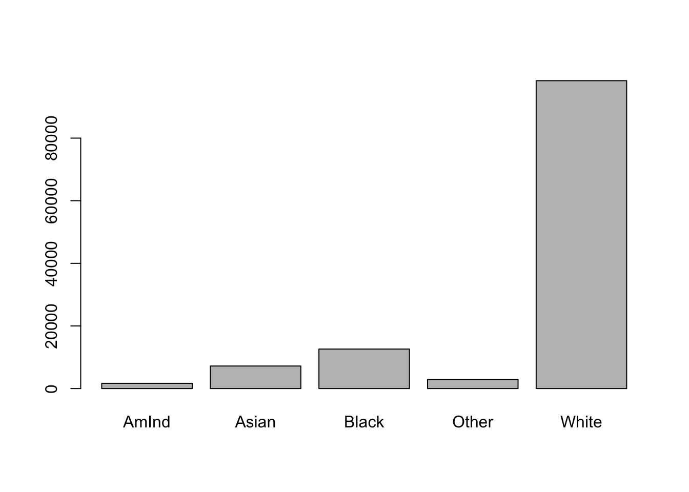
Generally, individuals are grouped into larger categories, and most typically those would be White, Black, Asian, Latino/Latina (if it’s available) and Other/Mixed Race. Sometimes American Indians are included as a separate category, other times they’re grouped in with “Other”. When you have small numbers of a given category it becomes really difficult to estimate differences between them and larger groups, and so sometimes you’re just forced to combine with another category. Let’s start by coding Whites, Blacks, and American Indians below since those are the first three categories shown in our code book.
dat$White <- ifelse(dat$RACE==100, 1, 0)
dat$Black <- ifelse(dat$RACE==200, 1, 0)
dat$AmInd <- ifelse(dat$RACE==300, 1, 0)
table(dat$White)
##
## 0 1
## 24400 98344##
## 0 1
## 110128 12616##
## 0 1
## 121071 1673This is a good moment to say that in creating new variable names you want to do two things: make it recognizable for yourself and short. The more characters you include, the more you will have to type later when you use it. But if I just name the variable for Whites “W” I might not remember what that is later. It’s a balancing act. Some names just become intuitive from practice. I didn’t make up the name AmInd for American Indians, it’s something I’ve seen elsewhere in data so I learned to use it myself. So make sure your new variable names are concise and clea.
What do we want to do with those that are coded as “Asian only” (651) and “Hawaiian/Pacific Islander only” (652). Do we want to combine them or leave them separate? Honestly, that is going to be determined by your research question and how central differences between different racial groups are for your analysis, as well as the amount of data you have. Here, I’ll code them both ways just for extra practice.
dat$Asian <- ifelse(dat$RACE==651|dat$RACE==652, 1, 0)
dat$AsianOnly <- ifelse(dat$RACE==651, 1, 0)
dat$HIPI <- ifelse(dat$RACE==652, 1, 0)
table(dat$Asian)
##
## 0 1
## 115546 7198##
## 0 1
## 116093 6651##
## 0 1
## 122197 547What that leaves is a lot of categorizations for either Other or combinations of different races. Again, it’s possible that your research will dictate that these should be left separate, but often we’ll want to combine those into a single category. Here we can do that by just asking whether the variable RACE is greater than 800.
5.3 Stacking ifelse
Above we have created 7 new variables denoting people’s races (although we created Asian in a few different ways) as a series of 0’s and 1’s. We can also create a new variable using words for the categories like we did in the variable Gender above by stacking ifelse() statements. Let’s jump into creating the first two values so we can talk in more detail about what we’re doing.
dat$RACE2 <- ifelse(dat$RACE==100, "White", NA)
dat$RACE2 <- ifelse(dat$RACE==200, "Black", dat$RACE2 )
In the first statement we ask if RACE equals 100, and set those values equal to “White” in our new variable. For the values that aren’t 100 we set them equal to NA, because we’ll fill their values in later. With the second ifelse() we set the values of 200 equal to “Black”, but we don’t want to overwrite the ones we made “White” in the first command for those that don’t equal 200 we want to leave them with their previous value of RACE2. That becomes more important as we stack on more values, and we want to create all of this within a single variable (Race2).
dat$RACE2 <- ifelse(dat$RACE==300, "AmInd", dat$RACE2 )
dat$RACE2 <- ifelse(dat$RACE==651|dat$RACE==652, "Asian", dat$RACE2 )
dat$RACE2 <- ifelse(dat$RACE>800, "Other", dat$RACE2 )
table(dat$RACE2)
##
## AmInd Asian Black Other White
## 1673 7198 12616 2913 98344We would probably rather have 5 separate dummy variables if we were using this for a regression. But if we’re just creating a graph for this variable, it’s easier if they’re all just included in one column.
Thus, you might use one strategy for the graph you include in a paper, and then use a different set of variables (that have equivalent information later in your analyses). The strategies you’ll use in creating new variables will always be indicated by the analysis you’re attempting to conduct.