Chapter 4 Loading Data
Up to this point the book has used a lot of data that is built into R. Reading data that already exists in r is quite simple, we just need the data() command. But that command wont work if we’re loading data in that is saved to our computer. The data() command is great when we’re just getting started because R has so many easy and pre-cleaned data sets available, but eventually you’ll want to work with your own data. So how do we load that in?
There are a few different ways, depending on how the data is saved. R can read in a lot of different types of data, and it can also export data into a lot of different forms with a few different basic commands.
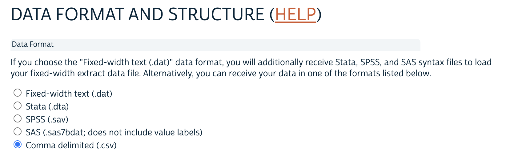
Why does data come in different forms? I don’t know. That’s all above my pay grade. Different websites you use to collect data will often give you different options, so it’s best to just sort of accept that you’re gonna have to be ready to work with it in different forms. When you’re given multiple options, I’d recommend choosing .csv. It’s the most flexible, it’s easy to open in excel if you want to look at it quickly, and you can open csv files in any software (not just R). As such, this chapter is going to go into the most depth on opening csv files. I’ll also provide the code to read in other types of data too, just for fun.
4.1 File Locations
It’s best if you practice loading in data along with the chapter. However, to do that you’ll need to have the same data files saved to your computer that I do. If you click on the following link it should take you to download 4 data files into a zip folder called RClass.
My suggestion would be to download those files and place the folder on your desktop, at least for the first round of practice if you haven’t loaded data into R from your computer before. you can move that folder somewhere else later as you get ore experienced, but that will make the examples done before more directly applicable. The folder will download as a zip to compress the files, so you’ll want to unzip them too, which usually just requires you to click on them.
Assuming you have the file saved, let’s talk about file locations. R is perfectly willing to open almost any file you might have on your computer, but you have to tell it where it is. You should imagine R as a helpful friend, but it can’t find anything for itself. You have to be very specific about where it should find what you want, and what you want. If you tell R you’d like it to get you a drink, it doesn’t know that “drinks” are typically in the fridge, or what constitutes a “drink.”
Figuring out the locations of files on our computer requires a little understanding of computers, and probably a better understanding of computers than I have. The data() command (which we’ve used elsewhere) works internally because it just looks with R to find the data that you list. When you want to read in external data that isn’t loaded into R you have to tell it where on your computer that data is saved. R has a default location that it’s going to look, which you can see where is with the command getwd().
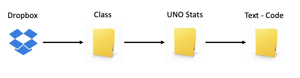
## [1] "/Users/evanholm/Dropbox/Class/UNO Stats/Text - Code"So currently my working directory is in a sub folder of my dropbox where I keep everything I’ve done related to this textbook.
This is a good time to run the getwd() command and see where R is operating out of on your computer.
If you want to change the folder R is using you can do that with setwd()
## [1] "/Users/evanholm/Dropbox/Class/UNO Stats"I’ve just moved my working directory one file back to the UNO Stats folder, rather than the textbook one. Let’s see what’s in my working directory.
##  [1] "_book"                 "_bookdown_files"
##  [3] "_bookdown.yml"         "_build.sh"
##  [5] "_deploy.sh"            "_output.yml"
##  [7] "01-introR.Rmd"         "02-sources.Rmd"
##  [9] "03-Loading.Rmd"        "04-ifelse.Rmd"
## [11] "05-Merging.Rmd"        "06-aggregate.Rmd"
## [13] "07-reducing.Rmd"       "08-markdown.Rmd"
## [15] "09-output.Rmd"         "bookdown-demo_files"
## [17] "Dockerfile"            "images"
## [19] "index.Rmd"             "LICENSE"
## [21] "now.json"              "README.md"
## [23] "rsconnect"             "style.css"
## [25] "toc.css"               "WorkingWithData_files"
## [27] "WorkingWithData.Rmd"
That shouldn’t mean much to you, it’s just a list of the different files that are in my working directory on my computer.
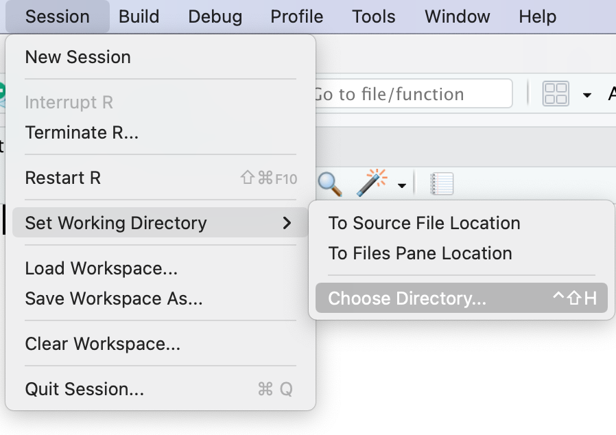
You can also set the working directory by pointing and clicking. At the top of the screen you can click on session, then Set Working Directory, then choose directory. There you can click through the folders on your computer and select exactly where you want R to operate, which should be wherever you’ve saved folders to.
My recommendation would be to create a folder on your desktop called RClass, where we’ll create and save files in this chapter. You can download the folder I’m using in this example using this link. That’s the same folder as above, just wanted to give everyone a second chance. If you already have a folder on your computer for this class that’s great, just figure out where that is saved and use its name and you can copy the individual files into it. I’m going to refer to a folder called RClass for the rest of this chapter to try and make things easier. I’m going to do that now on my own computer.
If you’re on a mac, the file directory actually gets a little easier. Rather than entering /Users/evanholm you can actually just use the tildy mark. I’m not sure why, but it’s one thing that makes using a mac a little easier. You’ll see me use the tildy mark in the rest of the examples in this chapter.
What if you’re not using a mac? The location of files should be similar, but you’ll need to figure out where it is. I would love to give you examples on a pc and mac, but unfortunately I can only record videos on my mac. On my pc this would be the file location.
setwd(“C:/Users/evanholm/Desktop/RClass”)
One more note. R uses forward slashes (“/”) rather than backslashes (""). That can be annoying, especially if you look up a file location manually on your computer. R will not recognize backslashes, only forward slashes.
Once we’ve changed our working directory that now becomes the location where R will look for our files. We can also read in our files by listing their locations below. If you want to practice and copy the code below, you’ll need to update the file locations to match what is on your computer.
Before we continue, let’s look at the files that are in that folder.
##  [1] "_book"                 "_bookdown_files"
##  [3] "_bookdown.yml"         "_build.sh"
##  [5] "_deploy.sh"            "_output.yml"
##  [7] "01-introR.Rmd"         "02-sources.Rmd"
##  [9] "03-Loading.Rmd"        "04-ifelse.Rmd"
## [11] "05-Merging.Rmd"        "06-aggregate.Rmd"
## [13] "07-reducing.Rmd"       "08-markdown.Rmd"
## [15] "09-output.Rmd"         "bookdown-demo_files"
## [17] "Dockerfile"            "images"
## [19] "index.Rmd"             "LICENSE"
## [21] "now.json"              "README.md"
## [23] "rsconnect"             "style.css"
## [25] "toc.css"               "WorkingWithData_files"
## [27] "WorkingWithData.Rmd"
4.2 CSV
CSV stands for comma separated values, which is a really common format for data that can work between different software programs. A CSV file is a plain text file that contains a list of data, with each value in a comma separated by a comma. R is able to read a csv in without loading any packages (which is one of the reasons I prefer it). We can use the command to load a file read.csv().
##   YEAR SERIAL MONTH  HWTFINL       CPSID REGION STATEFIP METRO METAREA
## 1 2018      1    11 1703.832 2.01708e+13     32        1     2    3440
## 2 2018      1    11 1703.832 2.01708e+13     32        1     2    3440
## 3 2018      3    11 1957.313 2.01809e+13     32        1     2    5240
## 4 2018      4    11 1687.784 2.01710e+13     32        1     2    5240
## 5 2018      4    11 1687.784 2.01710e+13     32        1     2    5240
## 6 2018      4    11 1687.784 2.01710e+13     32        1     2    5240
##   STATECENSUS FAMINC PERNUM   WTFINL      CPSIDP AGE SEX RACE EMPSTAT
## 1          63    830      1 1703.832 2.01708e+13  26   2  100      10
## 2          63    830      2 1845.094 2.01708e+13  26   1  100      10
## 3          63    100      1 1957.313 2.01809e+13  48   2  200      21
## 4          63    820      1 1687.784 2.01710e+13  53   2  200      10
## 5          63    820      2 2780.421 2.01710e+13  16   1  200      10
## 6          63    820      3 2780.421 2.01710e+13  16   1  200      10
##   LABFORCE EDUC VOTED VOREG
## 1        2  111    98    98
## 2        2  123    98    98
## 3        2   73     2    99
## 4        2   81     2    99
## 5        2   50    99    99
## 6        2   50    99    99
Again, you have to tell R exactly where that file is is saved. So let’s break that command down again, like we’re talking to a human.
“Hey R, can you grab me my file named cps_00003.csv, it’s on my computer, on the desktop, in the folder named RClass”.
Easy, R can understand that request.
4.3 DTA
read.csv() comes in base R, and it’s a really simply command to use. However, not all data is saved as a csv. Files saved for DAT are formatted to be read into a different statistical software called STATA. In order to read .dat files into R, we need to use a command in the package haven.
Be sure that haven is installed. If you get the error message Error in library(haven) : there is no package called ‘haven’, that means you need to run install.packages(“haven”) first before practicing the next chunk of code.
library(haven)
dat_dta <- as.data.frame(read_dta("/Users/evanholm/Desktop/RClass/cps_00003.dta"))
head(dat_dta)
## year serial month hwtfinl cpsid region statefip metro metarea
## 1 2018 1 11 1703.832 2.01708e+13 32 1 2 3440
## 2 2018 1 11 1703.832 2.01708e+13 32 1 2 3440
## 3 2018 3 11 1957.313 2.01809e+13 32 1 2 5240
## 4 2018 4 11 1687.784 2.01710e+13 32 1 2 5240
## 5 2018 4 11 1687.784 2.01710e+13 32 1 2 5240
## 6 2018 4 11 1687.784 2.01710e+13 32 1 2 5240
## statecensus faminc pernum wtfinl cpsidp age sex race empstat
## 1 63 830 1 1703.832 2.01708e+13 26 2 100 10
## 2 63 830 2 1845.094 2.01708e+13 26 1 100 10
## 3 63 100 1 1957.313 2.01809e+13 48 2 200 21
## 4 63 820 1 1687.784 2.01710e+13 53 2 200 10
## 5 63 820 2 2780.421 2.01710e+13 16 1 200 10
## 6 63 820 3 2780.421 2.01710e+13 16 1 200 10
## labforce educ voted voreg
## 1 2 111 98 98
## 2 2 123 98 98
## 3 2 73 2 99
## 4 2 81 2 99
## 5 2 50 99 99
## 6 2 50 99 99When using read_dat we also want to tell it we want to save what we’re loading as a data frame with the command as.data.frame().Notice what else changed above. The file location is the same, because both files are in the same folder. But I changed the file type (and the command). The new file I’m opening is saved as a .dta, not .csv. It has the same name and is in the same folder though.
4.4 SPSS
.sav is another file format that is specific to a certain statistical software: SPSS. Opening such a file will require yet another package too, foreign.
I don’t know why, but in order to open an SPSS file we also need to add to.data.frame=TRUE at the end of our command. I don’t know why, and I really don’t know why everyone can’t just save things as csv by default, but such is working with data.
library(foreign)
dat_sav <- read.spss("/Users/evanholm/Desktop/RClass/cps_00003.sav", to.data.frame = TRUE)
head(dat_sav)
## YEAR SERIAL MONTH HWTFINL CPSID REGION
## 1 2018 1 November 1703.832 2.01708e+13 East South Central Division
## 2 2018 1 November 1703.832 2.01708e+13 East South Central Division
## 3 2018 3 November 1957.313 2.01809e+13 East South Central Division
## 4 2018 4 November 1687.784 2.01710e+13 East South Central Division
## 5 2018 4 November 1687.784 2.01710e+13 East South Central Division
## 6 2018 4 November 1687.784 2.01710e+13 East South Central Division
## STATEFIP METRO METAREA STATECENSUS FAMINC PERNUM
## 1 Alabama Central city Huntsville,AL Alabama $60,000 - 74,999 1
## 2 Alabama Central city Huntsville,AL Alabama $60,000 - 74,999 2
## 3 Alabama Central city Montgomery, Al Alabama Under $5,000 1
## 4 Alabama Central city Montgomery, Al Alabama $50,000 - 59,999 1
## 5 Alabama Central city Montgomery, Al Alabama $50,000 - 59,999 2
## 6 Alabama Central city Montgomery, Al Alabama $50,000 - 59,999 3
## WTFINL CPSIDP AGE SEX RACE
## 1 1703.832 2.01708e+13 26 Female White
## 2 1845.094 2.01708e+13 26 Male White
## 3 1957.313 2.01809e+13 48 Female Black/Negro
## 4 1687.784 2.01710e+13 53 Female Black/Negro
## 5 2780.421 2.01710e+13 16 Male Black/Negro
## 6 2780.421 2.01710e+13 16 Male Black/Negro
## EMPSTAT LABFORCE
## 1 At work Yes, in the labor force
## 2 At work Yes, in the labor force
## 3 Unemployed, experienced worker Yes, in the labor force
## 4 At work Yes, in the labor force
## 5 At work Yes, in the labor force
## 6 At work Yes, in the labor force
## EDUC VOTED
## 1 Bachelor's degree No Response
## 2 Master's degree No Response
## 3 High school diploma or equivalent Voted
## 4 Some college but no degree Voted
## 5 Grade 10 Not in universe
## 6 Grade 10 Not in universe
## VOREG
## 1 Not reported / Not available
## 2 Not reported / Not available
## 3 Not in universe
## 4 Not in universe
## 5 Not in universe
## 6 Not in universeSee anything different in the data. The .sav file came with the different variable scoded with their different values; for instance, Race came with the different names, while it was numeric for the earlier versions. Why? I don’t know know. File formats are weird, but that’s a reason we want to check our data as it’s loading to make sure we understand what everything looks like under the good.
4.5 Dat
Another file format that is similar to .csv is .dat. You can read in such a file using the command read.table() if you ever come across it. I don’t often see it though, and it can get confusing because I name a lot of objects dat in R, and the file format is dat. read.table() is avaliable in base R without a package.
4.6 Excel
You can also read in excel files. I don’t recommend saving data in excel if you plan to use it in R though. Excel has a lot of great features for creating spreadsheets that are visibly appealing. But R doesn’t want visibly appealing data, it just wants the data. Let me pull a random example off the internet to talk about below. That’s something we discuss in more detail in another section on adding variables
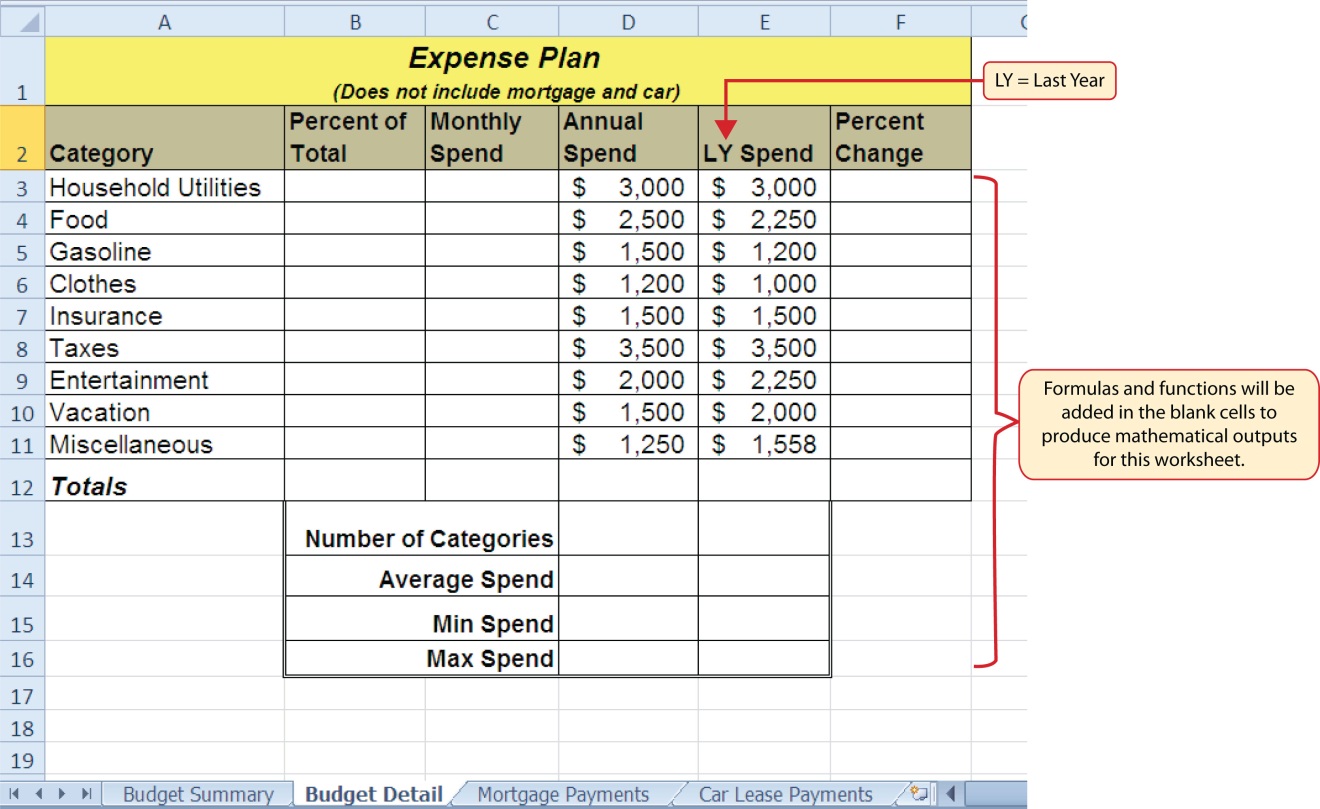
Wonderful, what a nicely organized spreadsheet. You can add formulas to calculate things across rows at the bottom, you’ve got color coded labels at the top. It’s beautiful. R would hate it.
R is going to look for the names of your columns along the top row, and will expect every column to have consistent information from top to bottom. Is that true for that spreadsheet above? No. The top row only says Expenses, so the file would read in with blank names for all of the columns but one. And when you get to the calculations at the bottom, those have nothing to do with the numbers above them.
I’m not criticizing anyone that uses Excel for these types of spreadsheets! It’s a great tool, but it’s not a great way to build data to read into R. That said, you still can. I’m not going to actually demonstrate it for you below because I want to get you out of the habit of using excel for data, but I’ll give you the code.
4.7 Writing Data
Along with reading in or loading data, we can also export or save our data. We can do that into many different formats, just like the way we can read it in from different formats, but I’m only going to focus on CSV. CSV is the simplest and cleanest way to load/save data, so if you’re saving the data yourself it’s the only thing you need to know initially.
Whereas we read in CSV data using read.csv, we can save it using write.csv. We just need to tell R what object we want to save, and where we want to save. See below.
If we want to save it to our working directory, we don’t need to put the full file location. Occasionally I do that and then discover my file is saved somewhere other than where I intended, so it’s best to just use the full file location.