Chapter 9 R Markdown Guide
9.1 What is Markdown
Markdown is an interactive system of text formatting that is a useful way to produce documents when using data and statistics. If you have ever produced a graph in Excel to put in a Word document, what do you have to do? Create the graph in excel, copy and paste it into Word, and probably redo the formatting to make it fit with the text. And if you decide to change the graph, you have to start all over again, adding each feature manually. R Markdown allows us to create the graph in our document using the R language, and automatically formats it. Over a lifetime of writing data-driven documents, it can save significant time and reduce the frustration of formatting and reformatting images. R Markdown is designed to make life easier for you.
By the way, everything you’re reading is written in R Markdown. I never could have completed this book if I had to manually insert all the graphs and functions that I will show you this semester. For instance, I probably saved 10 minutes on just this plot.
data(USJudgeRatings)
plot(USJudgeRatings$DECI, USJudgeRatings$PREP,
     main="Relationship Between Judge Preparation and Decisions",
     pch=16, col="blue")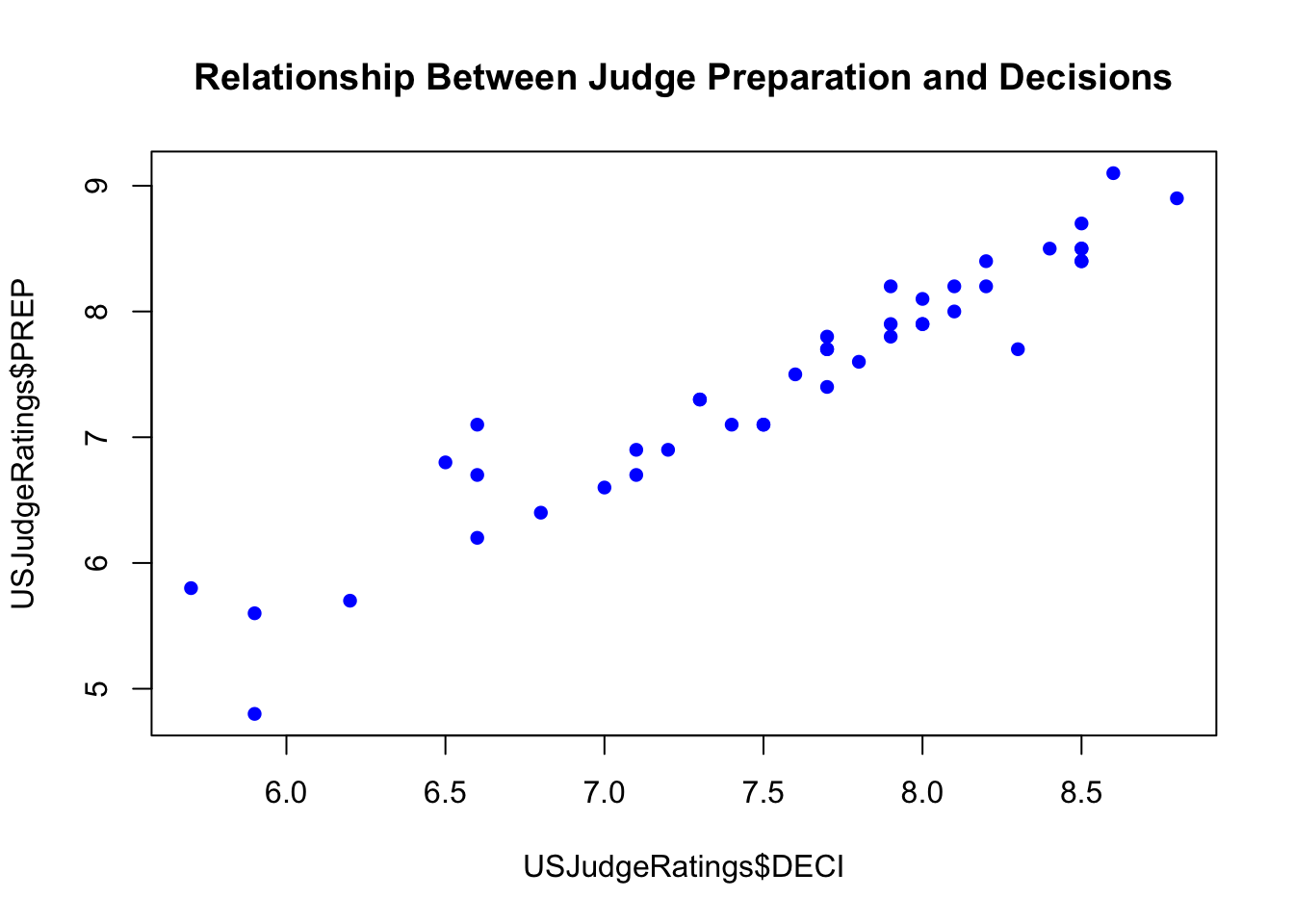
To try and explain Markdown a bit better, I’ll quote from Cosma Shalizi
You are probably used to word processing programs, like Microsoft Word, which employ the “what you see is what you get” (WYSIWYG) principle: you want some words to be printed in italics, and, lo, they’re in italics right there on the screen. You want some to be in a bigger, different font and you just select the font, and so on. This works well enough for n00bs but is not a viable basis for a system of text formatting, because it depends on a particular program (a) knowing what you mean and (b) implementing it well. For several decades, really serious systems for writing have been based on a very different principle, that of marking up text. The essential idea in a mark-up language is that it consists of ordinary text, plus signs which indicate how to change the formatting or meaning of the text. Some mark-up languages, like HTML (Hyper-Text Markup Language) use very obtrusive markup; others, like the language called Markdown, are more subtle.
We’ll explore that subtlety below later, but first let’s just get a brief tour of the mechanics of Markdown documents.
9.2 Getting Started
Let’s start with the basics. How to create an R Markdown document.
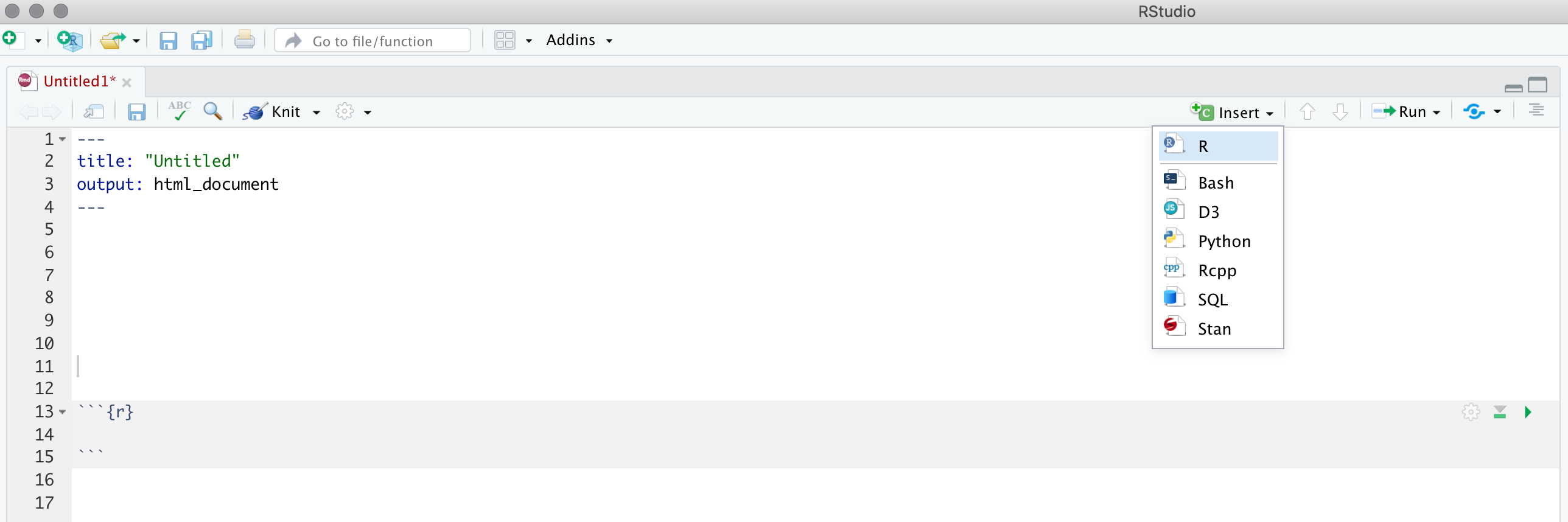
- Open R Studio
- Click on the upper left icon with white document and green plus sign.
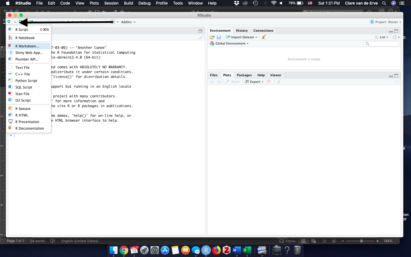
The first time you try to create a Markdown document you might be asked to install some other packages. Click yes. R knows what’s it is doing.
- In the drop down menu there is an option for R Markdown, click on it which will bring up a new screen.
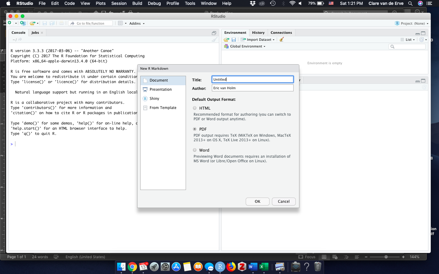 4. For now, let’s create our Markdown documents as PDFs. Enter any title you want and your name.
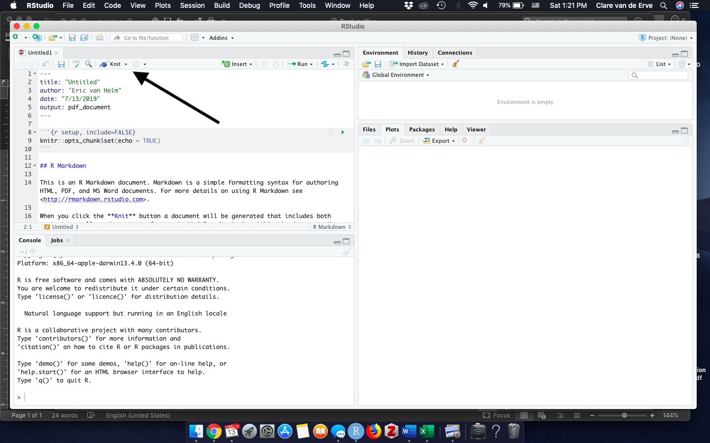
- Once you click OK, your new markdown will open with some sample code inserted. Let’s see what a finished R Markdown document looks like with that preset code.
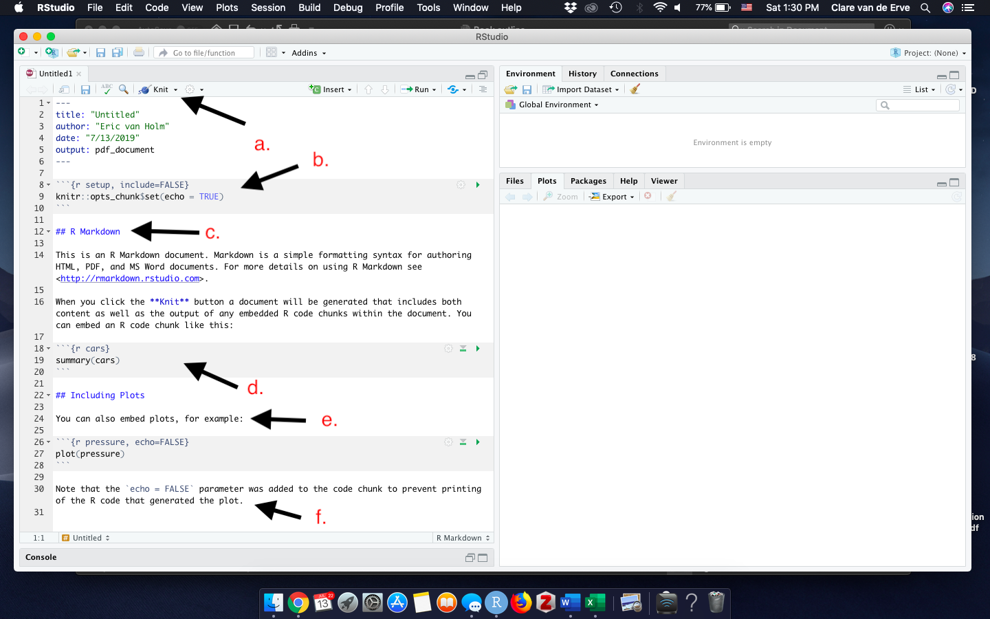
- The arrows highlight some important features to get us started.
- This is the knit button, which you’ll meet in a minute.
- This is code chunk. Much of what you write in a Markdown will just work as text, unless you put it in a code chunk. A code chunk starts with three ` (which are named back quotes, should be to the left of the numbers on your keyboard) and {r}. To close a code chunk you just put the three backquotes.That tells R that you’d like to write something in code, like printing a table or a graph. Otherwise, a Markdown document is just a written document and you can say something like 2 + 5 without it trying to create interpret that as a math statement.
- This is a heading. The reason that it shows in blue is because it isn’t just text, it has something added to it - the two hash tags that precede it means it will print larger and bold
- This is another code chunk
- This will print as plain text
- This final bit of text introduces an important feature of Markdown documents. if you insert echo=TRUE to your code chunk, the code you use will appear as part of the document, and if you write echo=FALSE it will not. If you’re writing a document that will be printed for the public, you might not want your code to show. If you’re turning in an assignment to your teacher, they’ll probably want to see your code.
To execute the Markdown document you need to press Knit, which will be in the upper middle of the screen. The first time you create a Markdown document as a pdf you’ll need to have the TinyTex package installed, so you will need to run this bit of code in R Studio tinytex::install_tinytex(). Enter that on the command line and execute it.
After you click Knit you’ll need to tell R where you want to save the document. If this was a part of an assignment you’d probably want to use a file you have for your class projects. For this document the desktop or downloads file will work. But anytime you Knit a Markdown document it will be saved.
Voila, you have created a Markdown document!
We’ll talk a lot more about the ways we can use R with Markdown this semester, and we’ll practice inserting code and graphs. For now, we need to focus on the text aspect of R Markdown. Some of this has been previewed above, but here I list many of the ways you can format your text in a Markdown document.
9.4 Code Chunks
Being able to insert a code chunk will become second nature, but it’s complicated at the start. We can write text in a Markdown, or we can write R Code. How does the Markdown know if we’re describing a plot “this plot is nice” versus trying to create a plot “plot(cars)”? It determines that by whether the text is in an R Code Chunk. Anything outside the chunk is processed as text, anything inside is processed as code. We want code inside the chunk, description outside. If you put regular text inside a code chunk and try to knit it will stop running because it wont be able to process the command “this plot is nice”. Code inside, description outside.
To insert a Code Chunk, look at the top of the document and there should be a green button labeled ‘insert’ Click it, click on the option R from the drop down menu, and a code chunk will be inserted.
The following video tries to make all of that clearer.
9.5 Why??
Why are we learning to write in Markdown? It can be a bit frustrating, but it makes inserting and formatting R output easier. Also, it makes inserting R code A LOT easier. For a class like this, that means I can see your code and output side by side on assignments. It takes a little learning, but it’s the quickest way to pull together text, code, and output. Again, that’s why I’ve used it to produce this entire book. How do you ensure that your code is displayed?
At the top of the R code chunk you can include “, echo=TRUE” which tells R that it should echo, or show, the code. You can also hide the code by saying echo=FALSE.
{r, echo=TRUE}Or you can include this at the top of the document, which tells Markdown to include code for all the chunks unless otherwise stated. This chunk comes with the Markdown document by default. You’ll want to clean out the default text that comes with the Markdown document, but you can generally leave this one.
knitr::opts_chunk$set(echo = TRUE)9.6 Proofing
One thing I still struggle with about writing in Markdown is the lack of automatic spellcheck. As you’ll probably notice reading these books, I occasionally make typos and I’m really bad at catching those myself. There is a spellcheck feature built into markdown (the little ABC with a checkmark at the top), but it’s not the best. It isn’t great at catching grammatical mistakes, and the dictionary is often missing words. And, it doesn’t even recognize R code as being spelled correctly, so it’ll ask you if every by.x= is spelled right. One thing I try to do when finishing a big document is copy it into Word to use its spellcheck, and I just ignore the misspellings in my code chunks since I’m just concerned with whether they work or not. Anyways, its an option.
9.7 Markdown Format Cheat sheet
This section describes and displays many of the most common formatting commands in Markdown. As I mentioned earlier, Markdown is part of the family of “markup” software, where you markup the document with formatting notes. So instead of typing a word and then clicking on bold to make it bold, you simply put a note in the text that you would like that word to be bolded. How we do that is described below.
9.7.1 Headers
# Heading One (h1)

## Heading Two (h2)

### Heading Three (h3)

#### Heading Four (h4)

##### Heading Five (h5)

###### Heading Six (h6)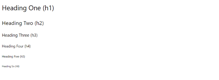
headings
9.7.2 Text Style
With Markdown, it is possible to emphasize words by making them *italicized*, using *astericks* or _underscores_, or making them **bold**, using **double astericks** or __double underscores__.

Of course, you can combine those two formats, with both _**bold and italicized**_ text, using any combination of the above syntax.

You can also add a strikethrough to text using a ~~double tilde~~.
With Markdown, it is possible to emphasize words by making them italicized, using asterisks or underscores, or making them bold, using double asterisks or double underscores.
Of course, you can combine those two formats, with both bold and italicized text, using any combination of the above syntax.
You can also add a strike through to text using a double tilde.
9.7.3 Lists
9.7.3.1 Unordered
* First item
* Second item
* Third item
    * First nested item
* Second nested item- First item
- Second item
- Third item
- First nested item
- Second nested item
9.7.3.2 Ordered
1. First item
2. Second item
3. Third item
    1. First nested item
2. Second nested item- First item
- Second item
- Third item
- First nested item
- Second nested item
9.7.4 Hyperlinks
Create links by wrapping the link text in square brackets [ ], and the URL in adjacent parentheses ( ).
[Google News](https://news.google.com)9.7.5 Images
Insert images in a similar way, but add an exclamation mark in front of square brackets [ ], and the image file name goes in the parentheses ( ).
The alt text appears when the image cannot be located, or is read by devices for the blind when the mouse hovers over the image. It
It is common practice to place all of the image files in an “assets” or “images” folder to keep your directory tidy. You can reference files inside a folder using the folder name and the forward slash:

credit: Shutterstock, but why?
Pictures are posted in their default size, which sometimes may be too large or small. If you want to scale them down or up, add { width= } to the end of the command.
{ width=50% }
Or you can link directly to an image online using the URL address of the image:

9.7.6 Tables
| Title 1          | Title 2          | Title 3         | Title 4         |
|------------------|------------------|-----------------|-----------------|
| First entry      | Second entry     | Third entry     | Fourth entry    |
| Fifth entry      | Sixth entry      | Seventh entry   | Eight entry     |
| Ninth entry      | Tenth entry      | Eleventh entry  | Twelfth entry   |
| Thirteenth entry | Fourteenth entry | Fifteenth entry | Sixteenth entry |
| Title 1 | Title 2 | Title 3 | Title 4 |
|---|---|---|---|
| First entry | Second entry | Third entry | Fourth entry |
| Fifth entry | Sixth entry | Seventh entry | Eight entry |
| Ninth entry | Tenth entry | Eleventh entry | Twelfth entry |
| Thirteenth entry | Fourteenth entry | Fifteenth entry | Sixteenth entry |
9.7.7 Blockquotes
9.7.7.1 Single line
> The purpose of life is to contribute in some way to making things better. - Robert F. KennedyThe purpose of life is to contribute in some way to making things better. - Robert F. Kennedy
9.7.7.2 Multiline
> Every time we turn our heads the other way when we see the law flouted, when we tolerate what we > know to be wrong, when we close our eyes and ears to the corrupt because we are too busy or too > frightened, when we fail to speak up and speak out, we strike a blow against freedom and decency > and justice.
>
> – Robert F. Kennedy
Each time a man stands up for an ideal, or acts to improve the lot of others, or strikes out against injustice, he sends forth a tiny ripple of hope, and crossing each other from a million different centers of energy and daring, those ripples build a current that can sweep down the mightiest walls of oppression and resistance.
-Robert F Kennedy
9.7.8 Horizontal Rule
---