Chapter 7 Changing Levels
Oftentimes you’ll want to use data from one unit of analysis to estimate a value at another unit of analysis. For instance, data from IPUMS is at the individual level, but it is often employed to make estimates about the characteristics of State’s or metropolitan area’s. So how do we transform data from one unit of analysis to another?
7.1 Movin’ On Up
Let’s start with a simplified example and some fictional data on counties within states. To keep this simple, we have information on the population of different counties. There are just 2 states in the data, and those 2 states have 4 and 3 counties to keep the example straightforward.
set.seed(5)
State <- c(1,1,1,1,2,2,2) # unique ID for each entry
County <- c(1,2,3,4,1,2,3)
Population<- round(rnorm(7, 450000, 50000),0) # median income
df1 <- data.frame(State,County,Population)
df1
## State County Population
## 1 1 1 407957
## 2 1 2 519218
## 3 1 3 387225
## 4 1 4 453507
## 5 2 1 535572
## 6 2 2 419855
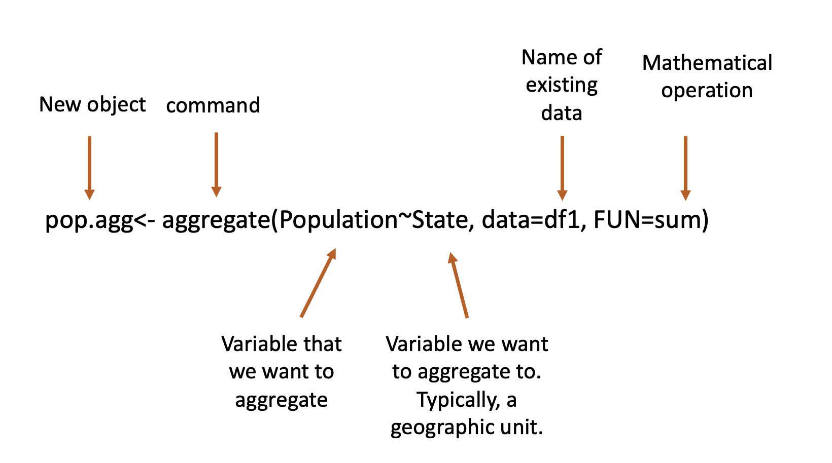
## 7 2 3 426392What I would like to get is the total population of the state based on the various values for counties. I can do that with the aggregate() command.
##   State Population
## 1     1    1767907
## 2     2    1381819
Let me annotate that command below.
We can do more than take the sum with the aggregate command. We can find the median…
##   State Population
## 1     1     430732
## 2     2     426392
Or the mean….
##   State Population
## 1     1   441976.8
## 2     2   460606.3
We can also aggregate our data at multiple levels at the same time. For instance, let’s say we have data for counties in states for multiple years, like below.
set.seed(5)
State <- c(3,3,3,3,4,4,4,3,3,3,3,4,4,4) # unique ID for each entry
County <- c(1,2,3,4,1,2,3,1,2,3,4,1,2,3)
Year <- c(2005,2005,2005,2005,2005,2005,2005, 2006,2006,2006,2006,2006,2006,2006)
Population<- round(rnorm(14, 450000, 50000),0) # median income
df2 <- data.frame(State,County,Year, Population)
df2
## State County Year Population
## 1 3 1 2005 407957
## 2 3 2 2005 519218
## 3 3 3 2005 387225
## 4 3 4 2005 453507
## 5 4 1 2005 535572
## 6 4 2 2005 419855
## 7 4 3 2005 426392
## 8 3 1 2006 418231
## 9 3 2 2006 435711
## 10 3 3 2006 456905
## 11 3 4 2006 511382
## 12 4 1 2006 409911
## 13 4 2 2006 395980
## 14 4 3 2006 442123To get the total population for each state IN EACH YEAR we just need to add a plus sign and the name of the additional variable we want accounted for.
##   State Year Population
## 1     3 2005    1767907
## 2     4 2005    1381819
## 3     3 2006    1822229
## 4     4 2006    1248014
7.2 Weights
So the aggregate command allows us to estimate the values for higher levels of analysis. It can’t guarantee that our estimates will be accurate though. Let’s once again go back to the data we used in previous sections from the Current Population Survey.
##   YEAR SERIAL MONTH  HWTFINL       CPSID REGION STATEFIP METRO METAREA
## 1 2018      1    11 1703.832 2.01708e+13     32        1     2    3440
## 2 2018      1    11 1703.832 2.01708e+13     32        1     2    3440
## 3 2018      3    11 1957.313 2.01809e+13     32        1     2    5240
## 4 2018      4    11 1687.784 2.01710e+13     32        1     2    5240
## 5 2018      4    11 1687.784 2.01710e+13     32        1     2    5240
## 6 2018      4    11 1687.784 2.01710e+13     32        1     2    5240
##   STATECENSUS FAMINC PERNUM   WTFINL      CPSIDP AGE SEX RACE EMPSTAT
## 1          63    830      1 1703.832 2.01708e+13  26   2  100      10
## 2          63    830      2 1845.094 2.01708e+13  26   1  100      10
## 3          63    100      1 1957.313 2.01809e+13  48   2  200      21
## 4          63    820      1 1687.784 2.01710e+13  53   2  200      10
## 5          63    820      2 2780.421 2.01710e+13  16   1  200      10
## 6          63    820      3 2780.421 2.01710e+13  16   1  200      10
##   LABFORCE EDUC VOTED VOREG
## 1        2  111    98    98
## 2        2  123    98    98
## 3        2   73     2    99
## 4        2   81     2    99
## 5        2   50    99    99
## 6 2 50 99 99## [1] 122744And let’s say we want to estimate the population of individual states using this data. Can we do that? We only have 122744 observations, but the population of the United States is much larger than that. This is why the data comes with “weights”, for exactly these types of calculations. The weights are calculated so that individual observations can approximate their size within the given population. A more detailed discussion of weights can be found here.
Let’s see what we’d estimate the population of the United States to be using the column WTFINL (weight final).
## [1] 323833483Those weights add up to 323,833,483. The United States population in 2018 was estimated to be 327.876 Million, so that’s really close! And, to be clear, that’s not an accident; that’s the point of the weights. Okay, let’s take a look at each individuals state’s population in 2018, as estimated by the CPS. The variable for state in that data is given by STATEFIP. We want to use the weight variable as the variable we want aggregated.
##   STATEFIP   WTFINL
## 1        1  4815491
## 2        2   709713
## 3        4  7059460
## 4        5  2971831
## 5        6 39335631
## 6        8  5616496
Let’s just check out math with the first state, Alabama (STATEFIP=1). We’ve estimated its population as 4,815,491. A quick Google search says that it’s population was 4.89 Million. That’s pretty close, but not exact. The CPS is just an approximation, but it’s going to give us close estimates for state level data and it’s margins of error should all be consistently close.
7.3 Merging Aggregations
Often times, when I need to aggregate one piece of data, I’ll want to add it back in to my original data. Notice that the column of data that’s generated for the total state population is the same as the name that was used for the individual weights in our original data. Let’s see what happens if I merge that back to my original data. I’d recommend reading the [section on merging] prior to going further. I’m going to create a subset of the data before going forward just to make this example a little clearer.
We can merge the state populations to the original data using STATEFIP which is in both sets of data. If you have the same variable with the same name in both sets of data you can just say by, rather than both by.x and by.y.
##   STATEFIP WTFINL.x WTFINL.y
## 1        1 1703.832  4815491
## 2        1 1845.094  4815491
## 3        1 1957.313  4815491
## 4        1 1687.784  4815491
## 5        1 2780.421  4815491
## 6        1 2780.421  4815491
Both sets of data had a column with the same name, so in order to distinguish them R added .x and .y to the end of the variable name. That’s a bit messy, especially since they hold really different information now. We can rename the columns either before or after our merge using the colnames() command to make sure our data remains clear.
##   STATEFIP   WTFINL State.Pop
## 1        1 1703.832   4815491
## 2        1 1845.094   4815491
## 3        1 1957.313   4815491
## 4        1 1687.784   4815491
## 5        1 2780.421   4815491
## 6        1 2780.421   4815491
That command renamed all of the columns in the data. We can also just rename on column by specifying the number of what we want to rename. Let’s rename the third column again to “ST.Pop”.
##   STATEFIP   WTFINL  ST.Pop
## 1        1 1703.832 4815491
## 2        1 1845.094 4815491
## 3        1 1957.313 4815491
## 4        1 1687.784 4815491
## 5        1 2780.421 4815491
## 6        1 2780.421 4815491
Okay, but let’s say we weren’t just interested in the total population in the state, but also what share of the population is college educated (or a given gender or gender or age groups, etc.). Do we have the tools to figure that out yet?
Let’s work on figuring out the gender breakdown of states. We have a variable for each respondents gender called SEX. Since there are only two levels to that variable, if we can figure out the share of women in a state, we’ll know the share of men as well (since it would just be 100- the percentage of women).
So let’s start by adding a new variable that accounts for whether the respondent is female. But, instead of making the value for the new variable 0 or 1, we’ll use the weights in the data, so that when we add up all of the females in the survey we’ll have an accurate proportion.
dat$Female <- ifelse(dat$SEX==2, dat$WTFINL, 0)

gender.agg <- aggregate(Female~STATEFIP, data=dat, FUN=sum)
head(gender.agg)
## STATEFIP Female
## 1 1 2502752
## 2 2 347774
## 3 4 3582658
## 4 5 1522759
## 5 6 19924925
## 6 8 2812541Okay, that’s an accurate count for how many women are in each state, but how do we figure out the percentage of women? We need to know the total number of people in each state then. So let’s do a second aggregate, and merge that into that same file.
##   STATEFIP   WTFINL
## 1        1  4815491
## 2        2   709713
## 3        4  7059460
## 4        5  2971831
## 5        6 39335631
## 6        8  5616496
gender.agg2 <- merge(gender.agg, pop.agg, by="STATEFIP")
colnames(gender.agg2) <- c("STATEFIP", "Females", "TotPop")
head(gender.agg2)## STATEFIP Females TotPop
## 1 1 2502752 4815491
## 2 2 347774 709713
## 3 4 3582658 7059460
## 4 5 1522759 2971831
## 5 6 19924925 39335631
## 6 8 2812541 5616496Now we just need to add a new variable for the percentage, which we can do by dividing the number of females by the total population.
##   STATEFIP  Females   TotPop    FemPct
## 1        1  2502752  4815491 0.5197293
## 2        2   347774   709713 0.4900206
## 3        4  3582658  7059460 0.5074975
## 4        5  1522759  2971831 0.5123976
## 5        6 19924925 39335631 0.5065363
## 6        8  2812541  5616496 0.5007644