Chapter 21 Samples and Distributions

21.1 Samples

Suppose you want R to pick lotto numbers for you. In Washington State, you get two plays for the cost of $1. That means, you get to pick two sets of 6 numbers from 1 to 49 for $1. To let R pick the lotto numbers, use the function, sample(x, n, replace) where

• x is the vector with elements drawm from either x or from integers 1:x
• n is the number of items to choose from and has to be a positive number
• replace = TRUE means sampling with replacement and replace = FALSE means sampling without replacement

Let us now pick our lotto numbers. We will call the first pick lotto1 and the second, lotto2.

lotto1 <- sample(49, 6, replace = FALSE)
lotto2 <- sample(49, 6, replace = FALSE)
lotto1

## [1] 12 33 26 16 49 24

lotto2

## [1] 47 31 35 11 30 28

21.2 Sampling Distribution

Let us look at the sampling distribution of the sample means to see how the Central Limit Theorem works. We will start with a uniform distribution.

unif <- c(1:8)
unif

## [1] 1 2 3 4 5 6 7 8

# Mean of our uniform distribution
mean(unif)

## [1] 4.5

# Standard deviation of our uniform distribution
sd(unif)

## [1] 2.44949

# Histogram
hist(unif, main = "Uniform Distribution", xlab = " ")

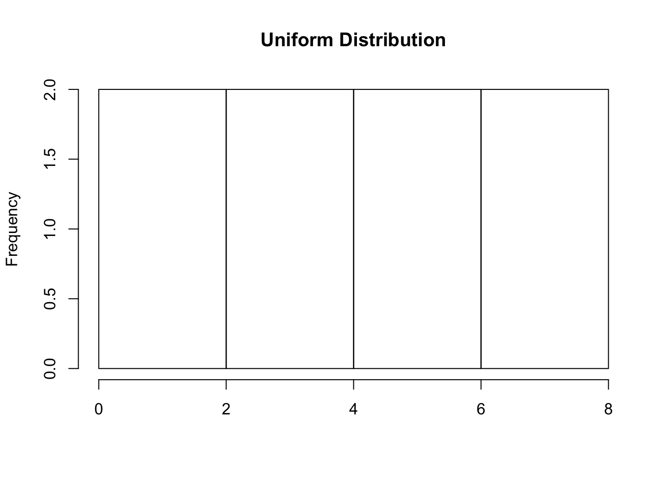
We will do a loop to keep calculating the sample mean of each sample taken. It is best to use a high number of repetitions. We will use 1000 here. We will also use the function, set. seed(seed) to ensure that the same result is gotten when any user starts with that same seed each time the same process is ran. The seed can be any single value.

set.seed(211)

# Sample size of 3
sample_means <- c( )
for(i in 1:1000){
        sample_means[i] <- mean(sample(8, 3, replace = TRUE))
}
hist(sample_means, xlim = c(0,8), main = "Sample Size of 3", xlab = "Sample Means")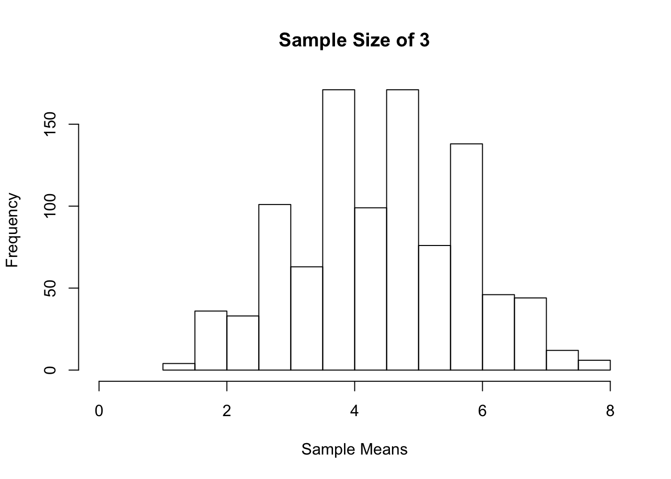

# Sample size of 10
for(i in 1:1000){
        sample_means[i] <- mean(sample(8, 10, replace = TRUE))
}
hist(sample_means, xlim = c(0,8), main = "Sample Size of 10", xlab = "Sample Means")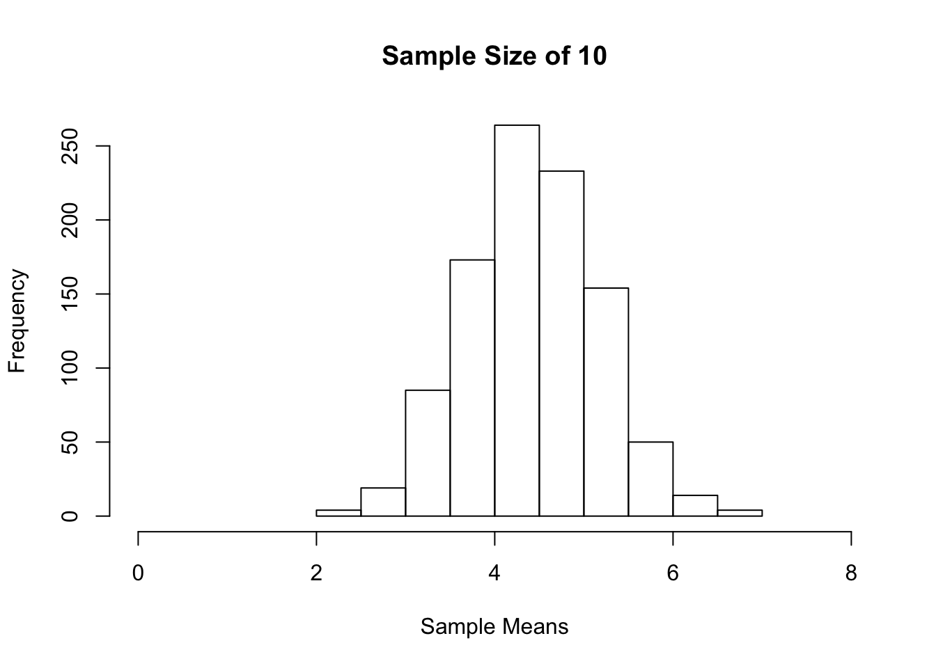

#Sample size of 30
for(i in 1:1000){
        sample_means[i] <- mean(sample(8, 30, replace = TRUE))
}
hist(sample_means, xlim = c(0,8), main = "Sample Size of 30", xlab = "Sample Means")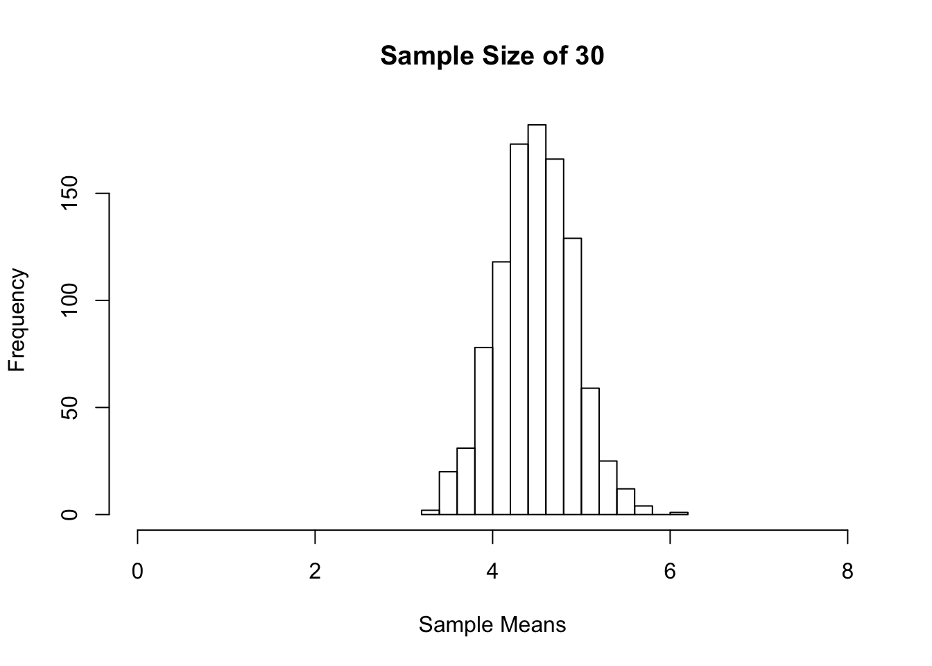

#Sample size of 50
for(i in 1:1000){
        sample_means[i] <- mean(sample(8, 50, replace = TRUE))
}
hist(sample_means, xlim = c(0,8), main = "Sample Size of 50", xlab = "Sample Means")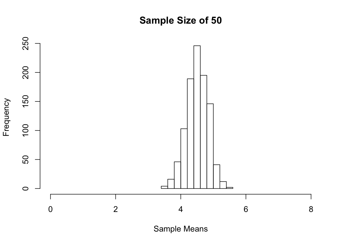

We started with a uniform distribution of the population 1 to 8. As the sample sizes got larger, we see that the sampling distribution of the sample mean became more symmetric. You can try the above using other distribution shapes. You will find that the sampling distribution of the sample mean becomes more symmetric as the sample size gets bigger.

21.3 Binomial Distribution

Let’s take a look at the binomial distribution. To create the binomial probability distribution, we will use the function, dbinom(x, size, prob) where x = vector of success, size = size of the sample, prob = probability of success. For graphing, we will use the function plot(x, y, type = “h”) where x = vector of success, y = dbinom( ) and type = “h” for histogram like vertical lines.

# Sample Size of 10
success <- c(0:10)
plot(success, dbinom(success, size = 10, prob = 0.25), 
     type = "h",
     main = "Sample Size of 10, p = 0.25",
     xlab = "Number of Successes",
     ylab = "Probability of Success",
     lwd = 3)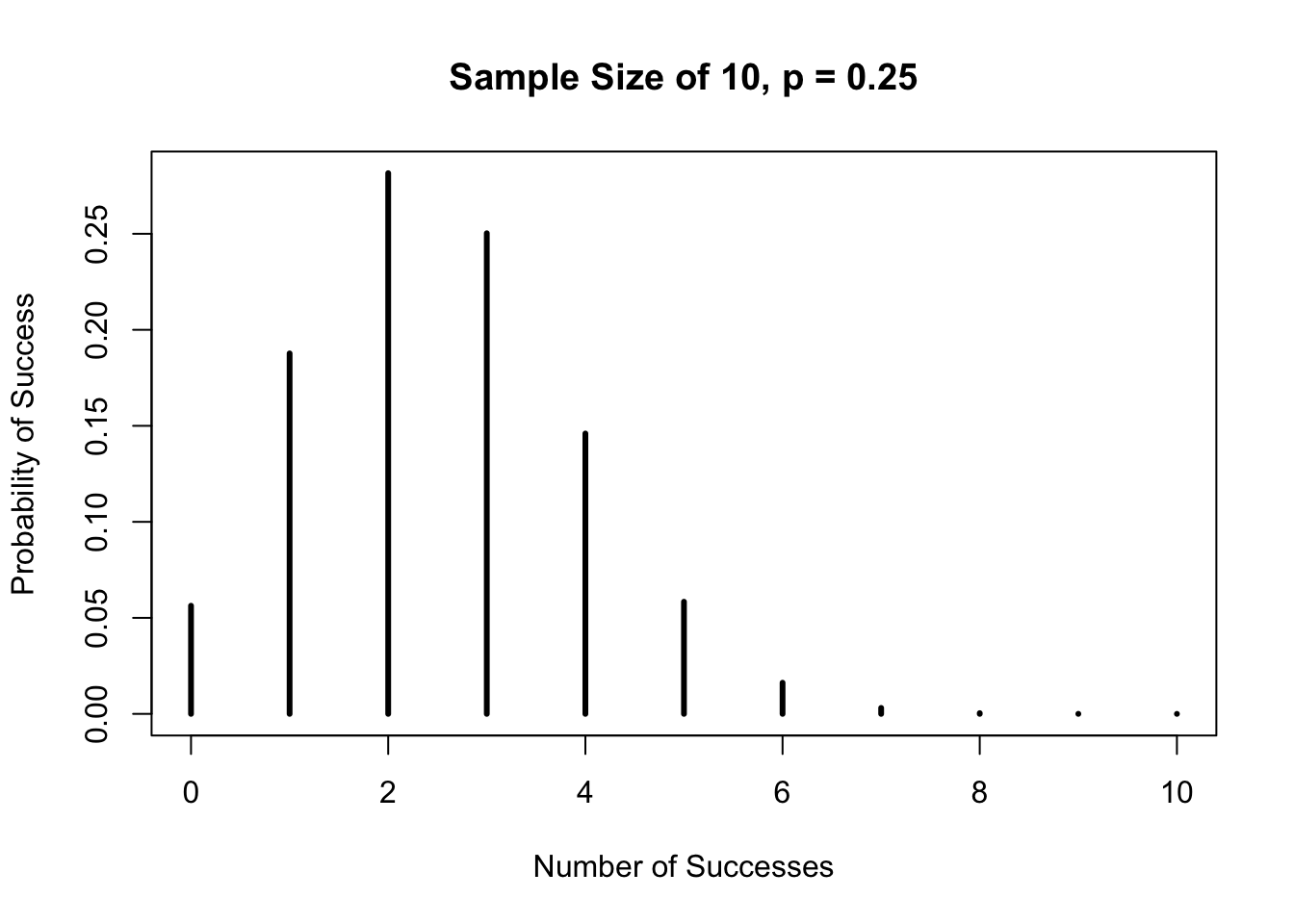

The distribution is right-skewed. However, as the sample size gets larger, the distribution becomes more symmetric as shown below.

# Sample Size of 30
suc <- c(0:30)
y <-  dbinom(suc, size = 30, prob = 0.25)
plot(suc, y, 
     type = "h",
     main = "Sample Size of 30, p = 0.25",
     xlab = "Number of Successes",
     ylab = "Probability of Success")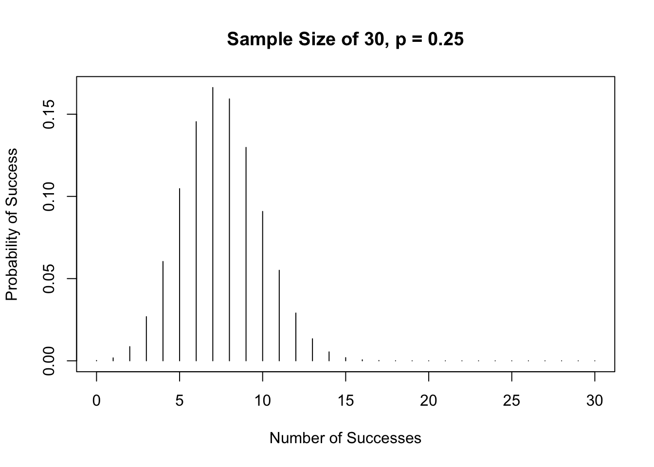

# Sample Size of 100
suc <- c(0:100)
y <-  dbinom(suc, size = 100, prob = 0.25)
plot(suc, y, 
     type = "h",
     main = "Sample Size of 100, p = 0.25",
     xlab = "Number of Successes",
     ylab = "Probability of Success")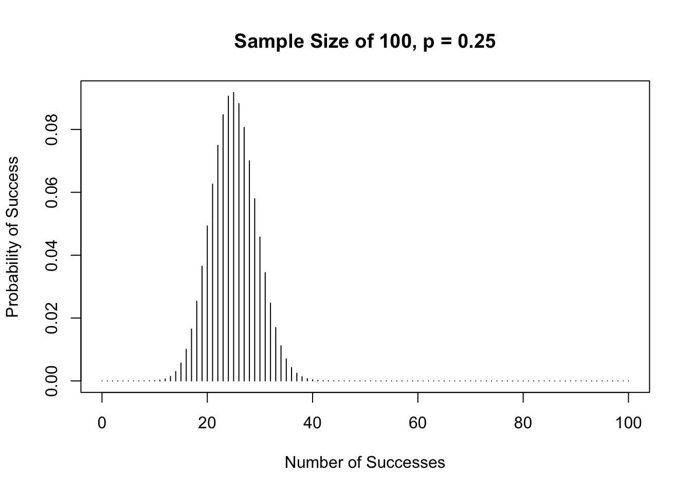

To calculate the probability of a binomial event, we will use either dbinom( ) or pbinom( ). The function dbinom( ) is similar to finding the probability of observing one particular event, ie, P(X = x) while pbinom gives the cumulative probability of an event, ie, P(X < x) or P(X <= x).

The arguments for both functions are basically the same: dbinom(x, size , prob) and pbinom(x, size, prob, lower.tail) where

• x = vector of success
• size is the sample size
• prob is the probability of success
• lower.tail = TRUE is the default; to get the upper-tail, set lower.tail = FALSE

Suppose a fair die is rolled 8 times. Success is if a “2” is rolled and failure is if all the other numbers are rolled. The probability of getting a “2” in one roll is 1/6 or 0.17. Let us take a look at the graph of this distribution.

success <- c(0:8)
plot(success, dbinom(success, size = 8, prob = 1/6), 
     type = "h",
     main = "Sample Size of 8, p = 1/6",
     xlab = "Number of Successes",
     ylab = "Probability of Success",
     lwd = 3)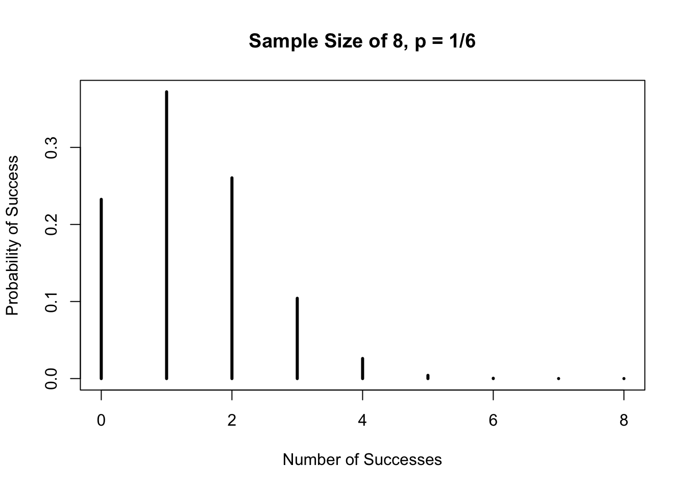

For each of the probability questions below, look at the graph above to see how the answers correlate.

a.) What is the probability of getting exactly three “2s” in eight rolls?

# P(X = 3)
dbinom(3, 8, 1/6)

## [1] 0.1041905

b.) What is the probability of getting three or less “2s” in eight rolls?

# P(X <= 3)
pbinom(3, 8, 1/6)

## [1] 0.9693436

c.) What is the probability of getting three or more “2s” in eight rolls?

# Using lower.tail = TRUE which is the default
# P(X >= 3) = 1 - P(X <= 2)
1 - pbinom(2, 8, 1/6)

## [1] 0.1348469

Using the upper-tail of the function, pbinom( ), is somewhat confusing. I suggest using the lower-tail all the time together with the idea of complement, if necessary.

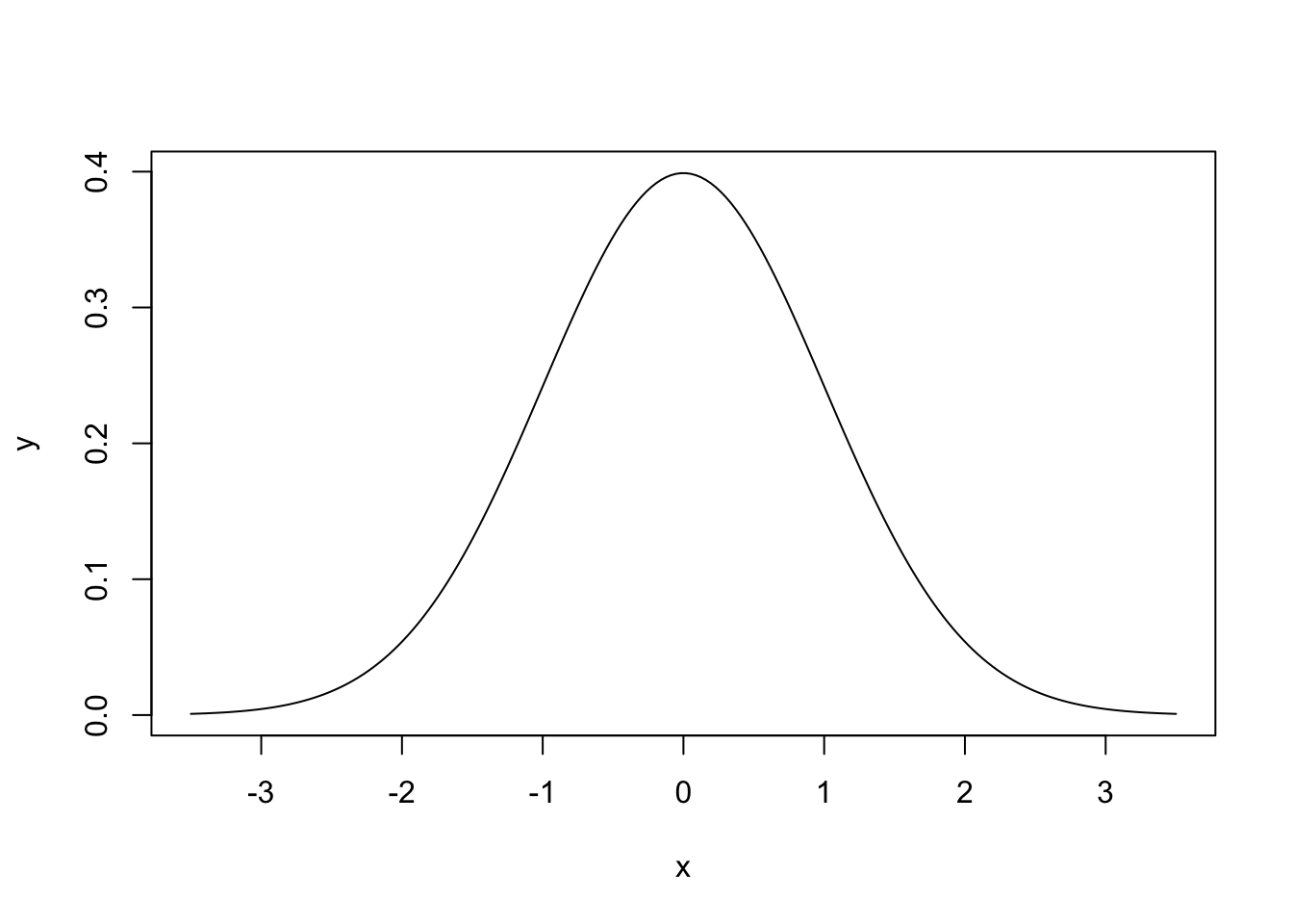
21.4 Normal Distribution

The normal distribution has a mean of 0 and standard deviation of 1. Its curve is bell-shaped, symmetric and unimodal as shown below.

To calculate probabilities, z-scores or tail areas of distributions, we use the function pnorm(q, mean, sd, lower.tail) where q is a vector of quantiles, and lower.tail = TRUE is the default.

Let us look at an example. On the normal curve, the area to the left of 0 with a mean of 0 and standard deviation of 1 is 0.5.

pnorm(0, 0, 1)

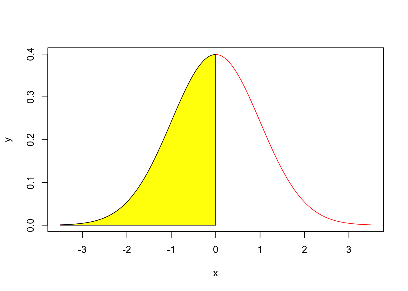
## [1] 0.5

If we want the area to the right of 1 on the normal curve, there are 2 ways to go about calculating this area.

# Using the upper-tail
pnorm(1, 0, 1, FALSE)

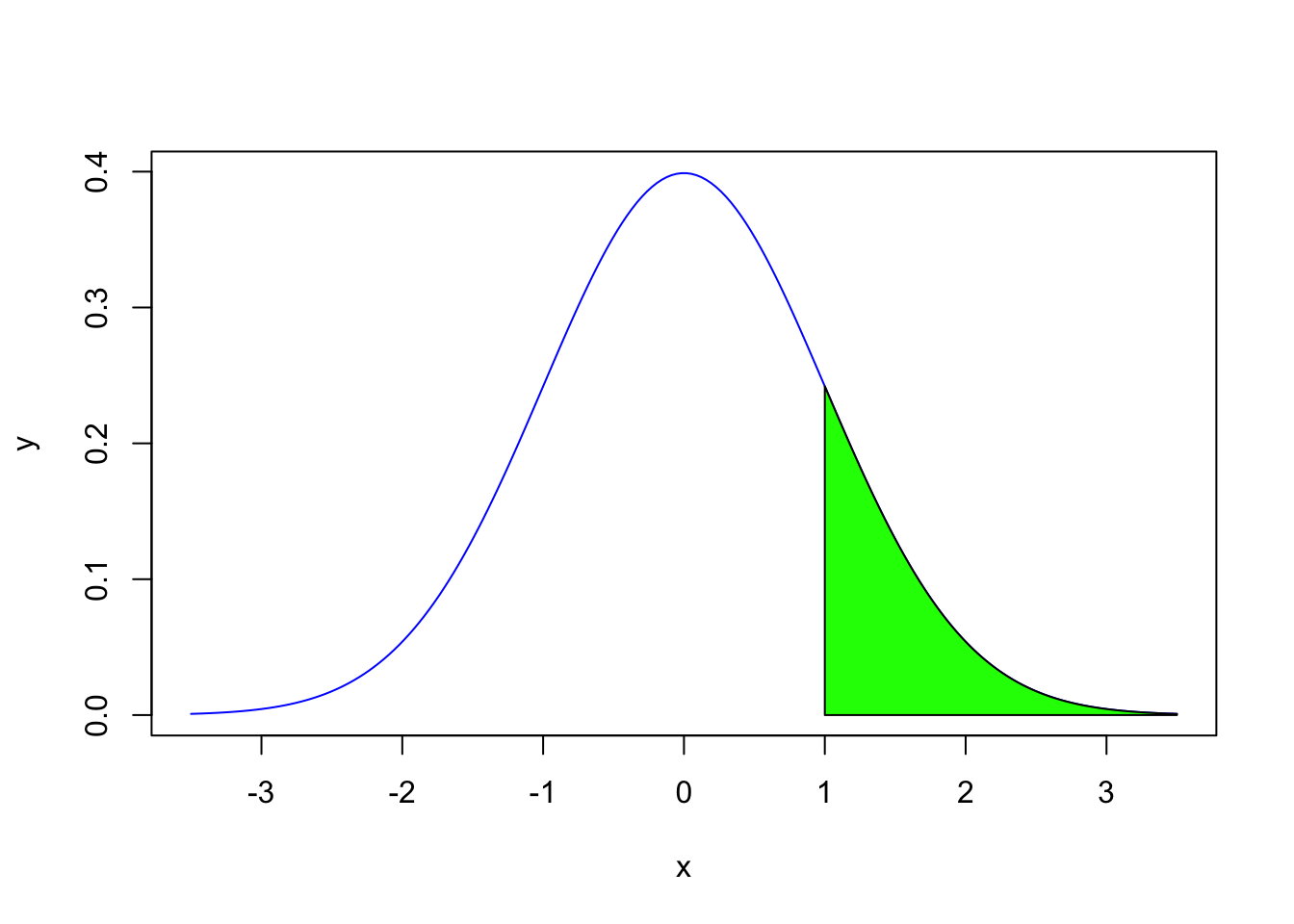
## [1] 0.1586553

# Using the lower-tail
1 - pnorm(1, 0, 1)

## [1] 0.1586553

Let’s take a look at an example where the mean is not at 0 and the standard deviation is not at 1. The heights of adult men in the United States are approximately normally distributed with a mean of 70 inches and a standard deviation of 3 inches.

a.) A man is randomly selected. His height is 72 inches. What percentile will he be?

pnorm(72, mean = 70, sd = 3)

## [1] 0.7475075

The man is almost in the 75th percentile.

b.) Suppose you want to find the probability of randomly selecting a man whose height is greater than 72 inches.

# We want the upper-tail
pnorm(72, mean = 70, sd = 3, FALSE)

## [1] 0.2524925

#We can also do a lower-tail
1 - pnorm(72, mean = 70, sd = 3)

## [1] 0.2524925

If you are given the probability and want to know a particular x-value, we use the function, qnorm(p, mean, sd, lower.tail) where p is the probability and lower.tail = TRUE is the default.

c.) Suppose a man is in the 40th percentile. How tall is this man?

qnorm(0.40, mean = 70, sd = 3)

## [1] 69.23996

The man is approximately 69 inches tall.