Chapter 16 Putting Everything Together
Let us review the functions used previously. Keep in mind, there are several ways to do a task. Multiple ways were shown previously but here, we will only show one way. It may not your preferred way. However, you are encouraged to try your preferred way and see if you get the same result.
16.1 Downloading Dataset
Let us take a look at a dataset that is found in this site: https://www.kaggle.com/ronitf/heart-disease-uci. Download the file heart.csv. Once the file is downloaded, upload it to RStudio by going to the Environment panel and clicking on the tab called Environment. Then click “Import Dataset”. A dropdown menu will appear. Choose “From Text (readr)…” Find your file and upload it to RStudio. You should now see your file in the Environment panel. Let us rename the file as heart.
Take a look at the first 6 lines of our dataset, heart.
##   age sex cp trestbps chol fbs restecg thalach exang oldpeak slope ca thal
## 1  63   1  3      145  233   1       0     150     0     2.3     0  0    1
## 2  37   1  2      130  250   0       1     187     0     3.5     0  0    2
## 3  41   0  1      130  204   0       0     172     0     1.4     2  0    2
## 4  56   1  1      120  236   0       1     178     0     0.8     2  0    2
## 5  57   0  0      120  354   0       1     163     1     0.6     2  0    2
## 6  57   1  0      140  192   0       1     148     0     0.4     1  0    1
##   target
## 1      1
## 2      1
## 3      1
## 4      1
## 5      1
## 6      1
There are 14 columns and the description of the headings of each column are as follows.
- age - age of patient in years
- sex - 0 for female and 1 for male
- cp - chest pain type (1 for typical angina, 2 for atypical angina, 3 for non-anginal pain and 4 for asymptmatic)
- trestbps - resting blood pressure on admission to the hospital (blood pressure is measured in mmHg)
- chol - cholesterol serum measured in mg/dl
- fbs - 0 for false and 1 for true if fasting blood sugar > 120 mg/dl
- restecg - resting electrocardiographic (ecg) results (0 for normal, 1 for having ST-T wave abnormality, 2 for showing probable or definite left ventricular hypertrophy)
- thalach - maximum heart rate achieved
- exang - 0 for No and 1 for Yes for exercise induced angina
- oldpeak - ST depression induced by exercise relative to rest
- slope - the slope of peak exercise ST segment
- ca - number of major vessels (0 - 3) colored by flourosopy
- thal - thallium stress test (1 for Fixed Defect, 2 for Normal, 3 for Reversible Defect)
- Target - diagnosis of heart disease (0 for < 50% and 1 for > 50% diameter narrowing in any major vessel)
16.2 Removing a Row
You can see the full dataset by using the function View(heart). A new tab called heart, will appear on the source panel showing the full dataset. There should be a total of 303 rows including the header row which is row 1.
If you go through the whole dataset slowly, you will notice that rows 164 and 165 are identical. Let us take a closer look at rows 160 to 170.
##     age sex cp trestbps chol fbs restecg thalach exang oldpeak slope ca thal
## 160  56   1  1      130  221   0       0     163     0     0.0     2  0    3
## 161  56   1  1      120  240   0       1     169     0     0.0     0  0    2
## 162  55   0  1      132  342   0       1     166     0     1.2     2  0    2
## 163  41   1  1      120  157   0       1     182     0     0.0     2  0    2
## 164  38   1  2      138  175   0       1     173     0     0.0     2  4    2
## 165  38   1  2      138  175   0       1     173     0     0.0     2  4    2
## 166  67   1  0      160  286   0       0     108     1     1.5     1  3    2
## 167  67   1  0      120  229   0       0     129     1     2.6     1  2    3
## 168  62   0  0      140  268   0       0     160     0     3.6     0  2    2
## 169  63   1  0      130  254   0       0     147     0     1.4     1  1    3
## 170  53   1  0      140  203   1       0     155     1     3.1     0  0    3
##     target
## 160      1
## 161      1
## 162      1
## 163      1
## 164      1
## 165      1
## 166      0
## 167      0
## 168      0
## 169      0
## 170      0
Notice that rows 164 and 165 have exactly the same entries. We do not want duplicate rows. Let us remove one of these rows.
##     age sex cp trestbps chol fbs restecg thalach exang oldpeak slope ca thal
## 160  56   1  1      130  221   0       0     163     0     0.0     2  0    3
## 161  56   1  1      120  240   0       1     169     0     0.0     0  0    2
## 162  55   0  1      132  342   0       1     166     0     1.2     2  0    2
## 163  41   1  1      120  157   0       1     182     0     0.0     2  0    2
## 165  38   1  2      138  175   0       1     173     0     0.0     2  4    2
## 166  67   1  0      160  286   0       0     108     1     1.5     1  3    2
## 167  67   1  0      120  229   0       0     129     1     2.6     1  2    3
## 168  62   0  0      140  268   0       0     160     0     3.6     0  2    2
## 169  63   1  0      130  254   0       0     147     0     1.4     1  1    3
## 170  53   1  0      140  203   1       0     155     1     3.1     0  0    3
## 171  56   1  2      130  256   1       0     142     1     0.6     1  1    1
##     target
## 160      1
## 161      1
## 162      1
## 163      1
## 165      1
## 166      0
## 167      0
## 168      0
## 169      0
## 170      0
## 171      0
Notice that the rows went from 163 to 165. Row 164 has now been removed. Be careful when you use numbers to call out a row. All the rows below row 164 have been shifted up. For example, row 165 as shown above is now row 164 when calling out in R, row 167 shown above is now row 166, etc.
Let us take a look at an example. Suppose we want to know the age of the study participant shown in row 168. As shown above, the age is 62. When calling out the row in R, you need to use row 167.
## [1] 62What if you enter 168 instead of 167?
## [1] 63The result is the age data for row 169.
16.3 Renaming a Variable
Suppose you want to change some of the variable names. For example, let us change the variable cp to chest_pain and trestbps to rest_bp.
names(heart)[names(heart) == "cp"] <- "chest_pain"
names(heart)[names(heart) == "trestbps"] <- "rest_bp"
head(heart)    # Check if changes were successful
## age sex chest_pain rest_bp chol fbs restecg thalach exang oldpeak slope ca
## 1 63 1 3 145 233 1 0 150 0 2.3 0 0
## 2 37 1 2 130 250 0 1 187 0 3.5 0 0
## 3 41 0 1 130 204 0 0 172 0 1.4 2 0
## 4 56 1 1 120 236 0 1 178 0 0.8 2 0
## 5 57 0 0 120 354 0 1 163 1 0.6 2 0
## 6 57 1 0 140 192 0 1 148 0 0.4 1 0
## thal target
## 1 1 1
## 2 2 1
## 3 2 1
## 4 2 1
## 5 2 1
## 6 1 116.4 Changing Data Entries
Suppose you want to change some of the data entries. For example, let us change the entries in the varaible, sex. Entry 0 will be changed to female and entry 1 to male. Let us also change the entries in the variable, exang. To indicate whether there was any angina induced by exercise or not, entry 0 will be changed to no and entry 1 to yes,
heart$sex[heart$sex == "0"] <- "female"
heart$sex[heart$sex == "1"] <- "male"
heart$exang[heart$exang == "0"] <- "no"
heart$exang[heart$exang == "1"] <- "yes"
head(heart)    # Check if changes were successful
## age sex chest_pain rest_bp chol fbs restecg thalach exang oldpeak slope ca
## 1 63 male 3 145 233 1 0 150 no 2.3 0 0
## 2 37 male 2 130 250 0 1 187 no 3.5 0 0
## 3 41 female 1 130 204 0 0 172 no 1.4 2 0
## 4 56 male 1 120 236 0 1 178 no 0.8 2 0
## 5 57 female 0 120 354 0 1 163 yes 0.6 2 0
## 6 57 male 0 140 192 0 1 148 no 0.4 1 0
## thal target
## 1 1 1
## 2 2 1
## 3 2 1
## 4 2 1
## 5 2 1
## 6 1 116.5 Categorical Variable Count
Let us look at the counts for categorical variables. Suppose we want to know how many male and female study participants there are.
##
## female   male
##     96    206
The result shows that there are 96 female and 206 male study participants.
##
##           no yes
##   female  74  22
##   male   129  77
The result shows that of the 96 female study participants, 74 had no exercise induced angina while 22 did. Of the 206 male study participants, 129 had no exercise induced angina while 77 did.
16.6 Statistics for Quantitative Variables
Let us look some statistics to describe the variable, rest_bp (resting blood pressure) of the participants.
## [1] 131.6026## [1] 17.56339## [1] 308.4728## [1] 94## [1] 200## [1] 130Let’s look at the summary statistics of the variable, thalach (maximum heart rate achieved).
##    Min. 1st Qu.  Median    Mean 3rd Qu.    Max.
## 71.0 133.2 152.5 149.6 166.0 202.0## [1] 71.0 133.0 152.5 166.0 202.0## [1] 32.75# For calculation to be more in line with our course, add the argument, type = 2
# Result shows Q3 - Q1 of fivenum( )
IQR(heart$thalach, type = 2)## [1] 33## [1] 71The summary( ) and fivenum( ) results are very similar. The IQR difference is not significant in this case. The IQR calculation using type = 2
16.7 Boxplot & Histogram
Let us draw a horizontal boxplot for the distribution of the maximum heart rate achieved and compare it to its histogram. Note that the default boxplot is vertical unless specified otherwise.
# Horizontal boxplot
boxplot(heart$thalach,
        horizontal = TRUE,
        main = "Boxplot of Maximum Heart Rate Achieved",
        xlab = "Maximum Heart Rate Achieved")
# Histogram
hist(heart$thalach,
     main = "Histogram of Maximum Heart Rate Achieved",
     xlab = "Maximum Heart Rate Achieved")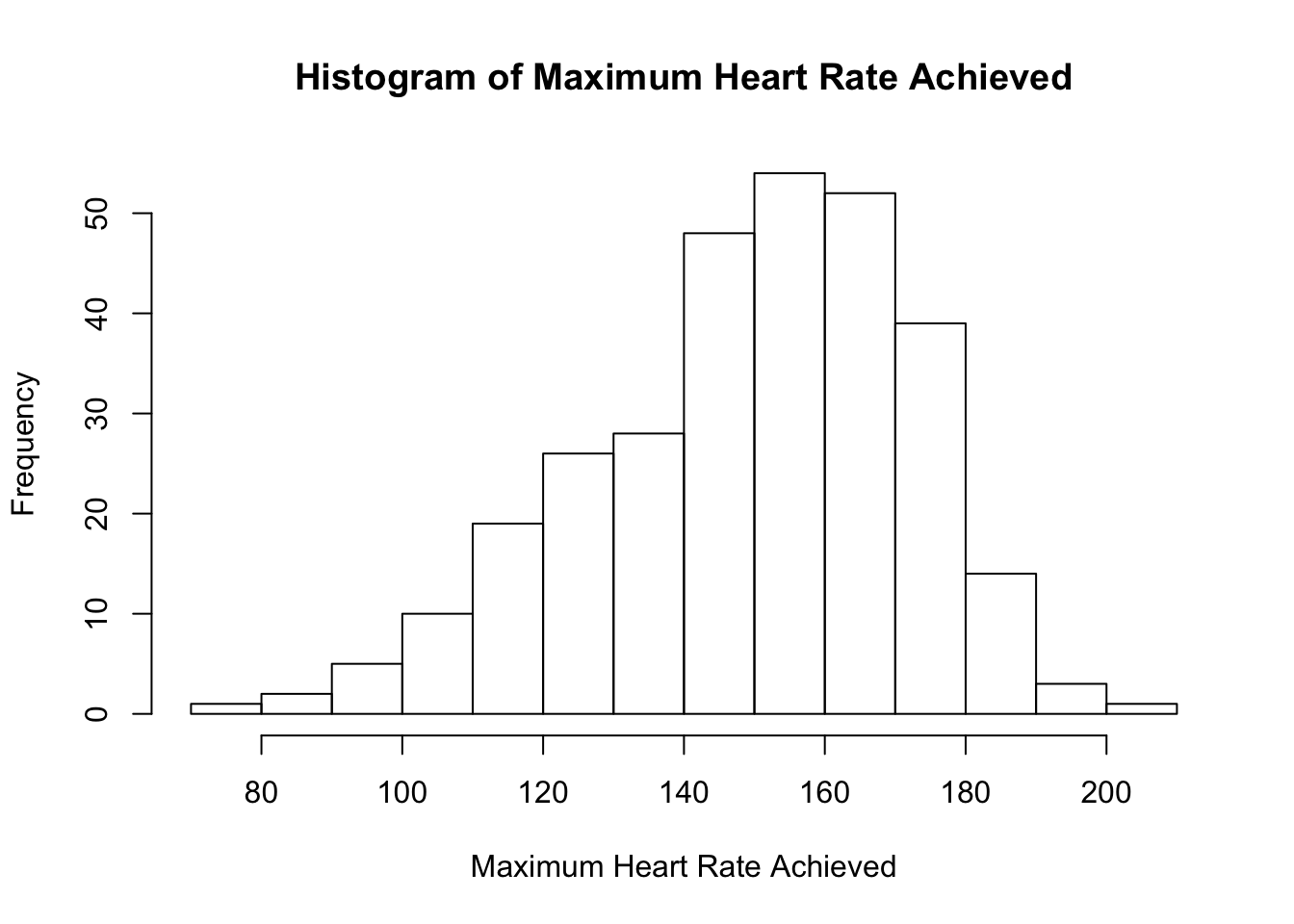
Both graphics show that the distribution for the maximum heart rate achieved is slightly left-skewed with potential outlier(s).
16.8 Dealing with Outliers
Let us now take a look at the boxplot and histogram of the variable, chol (cholesterol).
boxplot(heart$chol,
        horizontal = TRUE,
        main = "Boxplot of Cholesterol",
        xlab = "Cholesterol (in mg/dl)")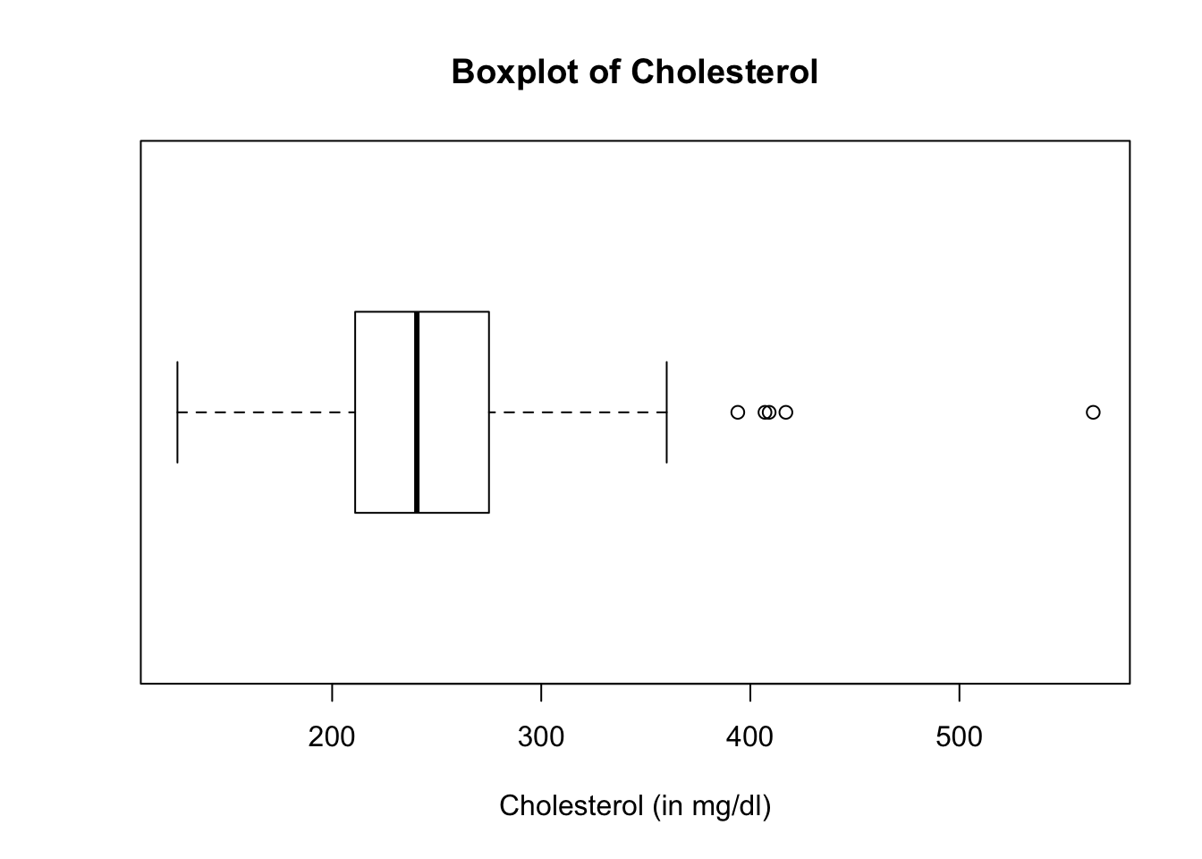
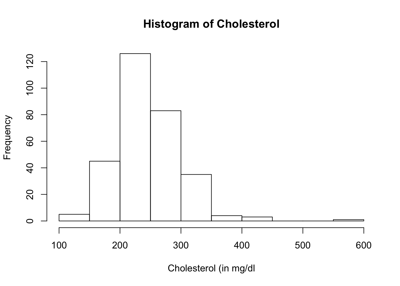
Both the boxplot and histogram of the the variable, chol, show several outliers. Let us extract the outliers.
## [1] 417 564 394 407 409