Chapter 24 Inference on Two Dependent Sample Means
We will be using the dataset called anorexia, in the package, MASS. This dataset looks at the weight changes of young female anorexia patients in 3 different treatment groups. The dataset shows the study participant’s weight before and after treatment. A hypothesis test will be done to assess if there is a statistically significant weight gain after treatment, regardless of treatment method.
24.1 Hypothesis Test Using Paired Values
Before we do the hypothesis test, let us first check that the assumptions are satisfied.
- The samples are randomly selected and paired.
- The sample size is large at n = 72.
- To check for outliers, we will draw the boxplot of the weight of the study participants. From below, the boxplots do not show any visible outliers.
boxplot(anorexia$Prewt, anorexia$Postwt,
        main = "Weight of Study Participants",
        names = c("Pre-Treatment", "Post Treatment"),
        ylab = "Weight (in pounds)")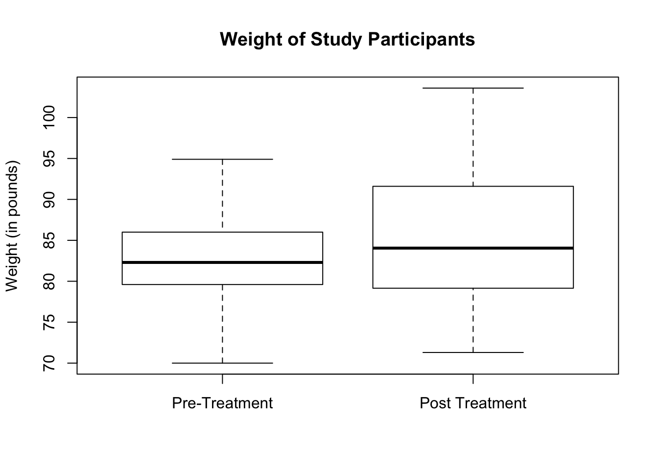
Additional arguments for t.test( ) may include the following:
- alternative = “two.sided”, “less”, or “greater”. If none is indicated, the argument defaults to two-sided.
- conf.level = confidence level desired. If none is indicated, the argument defaults to 95% confidence level.
In this example, we want to assess if the study participants have a statistically significant weight gain after treatment. A one-sided alternative test will be conducted. If the treatments were successful, then the difference between the variable, Prewt, which is the weight before the study, and the variable, Postwt, which is the weight after the study, will be less than 0. Be sure to include the argument, alternative = “less” in the t.test( ) function.
##
##  Paired t-test
##
## data:  anorexia$Prewt and anorexia$Postwt
## t = -2.9376, df = 71, p-value = 0.002229
## alternative hypothesis: true difference in means is less than 0
## 95 percent confidence interval:
##       -Inf -1.195825
## sample estimates:
## mean of the differences
##               -2.763889
The P-value is 0.002 which is quite small. The confidence interval, (-inf, -1.20), includes only negative numbers. That means, there is a statistically significant weight gain after treatment.
If you forgot the argument, alternative = “less”, then the test becomes a two-sided test. Let us take a look at the result.
##
##  Paired t-test
##
## data:  anorexia$Prewt and anorexia$Postwt
## t = -2.9376, df = 71, p-value = 0.004458
## alternative hypothesis: true difference in means is not equal to 0
## 95 percent confidence interval:
##  -4.6399424 -0.8878354
## sample estimates:
## mean of the differences
##               -2.763889
Notice that the t-statistic and degrees of freedom are the same as the one-sided test. However, the P-value of the two-sided test is double that of the one-sided test. Be aware of this result and remember to include the “alternative” argument if a one-sided test is intended.
If a confidence level different from 95% is desired, specify it using the argument conf.level.
##
##  Paired t-test
##
## data:  anorexia$Prewt and anorexia$Postwt
## t = -2.9376, df = 71, p-value = 0.002229
## alternative hypothesis: true difference in means is less than 0
## 90 percent confidence interval:
##       -Inf -1.546782
## sample estimates:
## mean of the differences
##               -2.763889
24.2 Hypothesis Test Using Value Differences
Alternatively, for a matched pair dataset, we can take differences of the variable entries and do a hypothesis test on the differences. To use value differences, we need to add a new column containing the differences between entries of our target variables. For this example, let us call the new variable (or column of differences), diff, which is the difference between entries in variable, Prewt, and variable, Postwt.
# Calculate a column of differences
diff <- anorexia$Prewt - anorexia$Postwt
# Append a new column called difference to the data frame
anorexia$diff <- diff
# Extract the first 6 lines of the data frame to show the new column
head(anorexia)
## Treat Prewt Postwt diff
## 1 Cont 80.7 80.2 0.5
## 2 Cont 89.4 80.1 9.3
## 3 Cont 91.8 86.4 5.4
## 4 Cont 74.0 86.3 -12.3
## 5 Cont 78.1 76.1 2.0
## 6 Cont 88.3 78.1 10.2Before we start the hypothesis test, let us check that the assumptions are satisfied.
- The samples are randomly selected and paired.
- The sample size is large at n = 72.
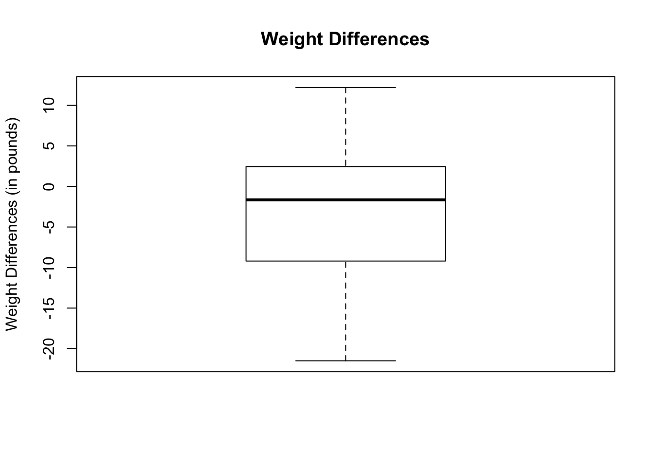
- To check for outliers, we will draw the boxplot of the weight differences. From below, the boxplot does not show any outliers.
Additional arguments for t.test( ) may include the following unless required is specified:
- alternative = “two.sided”, “less”, or “greater”. If none is indicated, the argument defaults to two-sided.
- conf.level = confidence level desired. If none is indicated, the argument defaults to 95% confidence level.
Note that mu does not have to be specified. The default is mu = 0.
In this example, we want to assess if the study participants have a statistically significant weight gain after treatment. If the treatments are successful, then the weight differences should be less than 0. A one-sided alternative test will be conducted. Be sure to include the argument, alternative = “less” in the t.test( ) function.
##
##  One Sample t-test
##
## data:  anorexia$diff
## t = -2.9376, df = 71, p-value = 0.002229
## alternative hypothesis: true mean is less than 0
## 95 percent confidence interval:
##       -Inf -1.195825
## sample estimates:
## mean of x
## -2.763889
The results are exactly the same as doing a matched pair hypothesis test using paired variables.