Chapter 15 Descriptive Statistics for Data Frame
We will work with the dataset built into R called chickwts. Note that chickwts is a data frame. This dataset shows the chick weight, in grams, 6 weeks after newly hatched chicks were randomly placed into six groups by feed type. The dataset has 2 variables, weight and feed. Variable weight is quantitative while variable feed is categorical.
15.1 Catergorical Variable Count
To get a count of a categorical variable, use the function, table(categorical_variable).
##
##    casein horsebean   linseed  meatmeal   soybean sunflower
##        12        10        12        11        14        12
15.2 Describing Distribution
Let us use the function, fivenum( ) to look at the five-number summary of the variable weight.
## [1] 108.0 204.5 258.0 323.5 423.0Notice that the result took all of the chick weights into consideration without regard to the feed type.
Let us now look at the function, summary( ).
##      weight             feed
##  Min.   :108.0   casein   :12
##  1st Qu.:204.5   horsebean:10
##  Median :258.0   linseed  :12
##  Mean   :261.3   meatmeal :11
##  3rd Qu.:323.5   soybean  :14
##  Max.   :423.0   sunflower:12
Notice that we get a five number summary, taking all of the chick weights into consideration. An additional column on feed shows the number of chicks on a particular feed type.
15.3 Describing Distribution by Group
What if we want to describe a distribution but grouped by feed type? To do so, we use the function, by( ) or aggregate( ). Both functions give the same result but present the results differently.
By( ) Function
The by( ) function syntax is: by(quantitative_variable, factor, function), where factor is the grouping variable desired.
Let’s look at the mean weight for each feed type.
## chickwts$feed: casein
## [1] 323.5833
## ------------------------------------------------------------
## chickwts$feed: horsebean
## [1] 160.2
## ------------------------------------------------------------
## chickwts$feed: linseed
## [1] 218.75
## ------------------------------------------------------------
## chickwts$feed: meatmeal
## [1] 276.9091
## ------------------------------------------------------------
## chickwts$feed: soybean
## [1] 246.4286
## ------------------------------------------------------------
## chickwts$feed: sunflower
## [1] 328.9167
Let’s look at the standard deviation of the weights grouped by feed type.
## chickwts$feed: casein
## [1] 64.43384
## ------------------------------------------------------------
## chickwts$feed: horsebean
## [1] 38.62584
## ------------------------------------------------------------
## chickwts$feed: linseed
## [1] 52.2357
## ------------------------------------------------------------
## chickwts$feed: meatmeal
## [1] 64.90062
## ------------------------------------------------------------
## chickwts$feed: soybean
## [1] 54.12907
## ------------------------------------------------------------
## chickwts$feed: sunflower
## [1] 48.83638
Let us take a look at the functions, summary( ) and fivenum( ). Remember that the quartiles are computed differently so you may see discrepancies in the first and third quartile results. Fivenum( ) computation is what we are more familiar with.
## chickwts$feed: casein
##    Min. 1st Qu.  Median    Mean 3rd Qu.    Max.
##   216.0   277.2   342.0   323.6   370.8   404.0
## ------------------------------------------------------------
## chickwts$feed: horsebean
##    Min. 1st Qu.  Median    Mean 3rd Qu.    Max.
##   108.0   137.0   151.5   160.2   176.2   227.0
## ------------------------------------------------------------
## chickwts$feed: linseed
##    Min. 1st Qu.  Median    Mean 3rd Qu.    Max.
##   141.0   178.0   221.0   218.8   257.8   309.0
## ------------------------------------------------------------
## chickwts$feed: meatmeal
##    Min. 1st Qu.  Median    Mean 3rd Qu.    Max.
##   153.0   249.5   263.0   276.9   320.0   380.0
## ------------------------------------------------------------
## chickwts$feed: soybean
##    Min. 1st Qu.  Median    Mean 3rd Qu.    Max.
##   158.0   206.8   248.0   246.4   270.0   329.0
## ------------------------------------------------------------
## chickwts$feed: sunflower
##    Min. 1st Qu.  Median    Mean 3rd Qu.    Max.
## 226.0 312.8 328.0 328.9 340.2 423.0## chickwts$feed: casein
## [1] 216.0 271.5 342.0 373.5 404.0
## ------------------------------------------------------------
## chickwts$feed: horsebean
## [1] 108.0 136.0 151.5 179.0 227.0
## ------------------------------------------------------------
## chickwts$feed: linseed
## [1] 141.0 175.0 221.0 258.5 309.0
## ------------------------------------------------------------
## chickwts$feed: meatmeal
## [1] 153.0 249.5 263.0 320.0 380.0
## ------------------------------------------------------------
## chickwts$feed: soybean
## [1] 158 199 248 271 329
## ------------------------------------------------------------
## chickwts$feed: sunflower
## [1] 226.0 307.5 328.0 340.5 423.0Aggregate( ) Function
The aggregate function syntax is:Let’s compute the median weight of each feed type.
##   Type of Feed     x
## 1       casein 342.0
## 2    horsebean 151.5
## 3      linseed 221.0
## 4     meatmeal 263.0
## 5      soybean 248.0
## 6    sunflower 328.0
Let’s compute the weight variance of each feed type.
##   Type of Feed        x
## 1       casein 4151.720
## 2    horsebean 1491.956
## 3      linseed 2728.568
## 4     meatmeal 4212.091
## 5      soybean 2929.956
## 6    sunflower 2384.992
Let’s look at the functions, summary( ) and fivenum( ). Remember that the quartiles are computed differently so you may see discrepancies in the first and third quartile results. Fivenum( ) computation is what we are more familiar with.
##   Type of Feed   x.Min. x.1st Qu. x.Median   x.Mean x.3rd Qu.   x.Max.
## 1       casein 216.0000  277.2500 342.0000 323.5833  370.7500 404.0000
## 2    horsebean 108.0000  137.0000 151.5000 160.2000  176.2500 227.0000
## 3      linseed 141.0000  178.0000 221.0000 218.7500  257.7500 309.0000
## 4     meatmeal 153.0000  249.5000 263.0000 276.9091  320.0000 380.0000
## 5      soybean 158.0000  206.7500 248.0000 246.4286  270.0000 329.0000
## 6 sunflower 226.0000 312.7500 328.0000 328.9167 340.2500 423.0000## Type of Feed x.1 x.2 x.3 x.4 x.5
## 1 casein 216.0 271.5 342.0 373.5 404.0
## 2 horsebean 108.0 136.0 151.5 179.0 227.0
## 3 linseed 141.0 175.0 221.0 258.5 309.0
## 4 meatmeal 153.0 249.5 263.0 320.0 380.0
## 5 soybean 158.0 199.0 248.0 271.0 329.0
## 6 sunflower 226.0 307.5 328.0 340.5 423.0From the above examples, we see that both the by( ) and aggregate( ) functions give the same results. However, the result presentation and function syntax are different.
15.4 Subsetting
In this dataset, there are numerous feed types. What if we are only interested in the one called sunflower? To focus on just sunflower, we will have to form a subset. This way, none of the other feed types are entered into the calculation. Let us call the subset, sunflower.
sunflower <- subset(chickwts, chickwts$feed == "sunflower")
sunflower # Lists elements in the subset
## weight feed
## 37 423 sunflower
## 38 340 sunflower
## 39 392 sunflower
## 40 339 sunflower
## 41 341 sunflower
## 42 226 sunflower
## 43 320 sunflower
## 44 295 sunflower
## 45 334 sunflower
## 46 322 sunflower
## 47 297 sunflower
## 48 318 sunflowerThe dataset, chickwts, has 71 rows. After forming the subset, sunflower, we now have 12 rows.
15.5 Dealing with Outliers
Let us draw the boxplot of the variable, weight, in the subset sunflower.
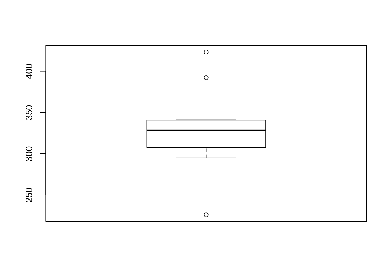
The boxplot shows three outliers. Let us compute these outliers.
The fastest way to compute outliers is to use the function, boxplot.stats( )$out.
## [1] 423 392 226Remember that the first and third quartiles are computed differently in boxplot.stats( ) than what we are more familiar with. Sometimes, we get outlier discrepancies.
We can use the function, fivenum( ), to calculate outliers. This method is longer but the result is in line with what we’re familiar with. We know that suspected outliers fall more than 1.5*IQR below Q1 or above Q3. To calculate IQR, we will use the type = 2.
## [1] 258## [1] 390Take a look at the five-number summary of the subset, sunflower, to see if we have any outliers.
## [1] 226.0 307.5 328.0 340.5 423.0The minimum value, 226, is smaller than the calculated lower inner fence of 258, and the maximum value, 423 is larger than the upper inner fence, 390. This means that there must be at least one outlier on either end.
In order to list the outliers, we need to make a subset of the subset, sunflower. We will call the subset containing all elements less than the lower inner fence, sunflower_lower and all the elements greater than upper inner fence, sunflower_upper
sunflower_lower <- subset(sunflower, sunflower$weight < 258)
sunflower_lower # Lists all elements below lower inner fence
## weight feed
## 42 226 sunflowersunflower_upper <- subset(sunflower, sunflower$weight > 390)
sunflower_upper # Lists all elements above upper inner fence## weight feed
## 37 423 sunflower
## 39 392 sunflowerUsing this method, we get more information on the outlier. In this case, aside from the outlier weight, we are also informed on the type of feed used and the row containing the outlier.