Chapter 22 Inference on One Sample Mean

Let us look at the dataset about rat genotype found in the package called MASS. We will focus on the variable, Wt, which is a rat litter’s average weight gain, in grams, at age 28 days.

# Load package MASS
library(MASS)

Let us take a look at some summary statistics for the variable, Wt.

# Five-number summary
fivenum(genotype$Wt)

## [1] 36.3 48.2 54.0 60.3 69.8

# Sample mean of weight gain
mean(genotype$Wt)

## [1] 53.97049

# Standard deviation of weight gain
sd(genotype$Wt)

## [1] 8.266526

# Length of vector
length(genotype$Wt)

## [1] 61

22.1 Check Distribution

Before doing a hypothesis test, check that the average weight gain distribution is approximately normal. Let us look at the histogram.

hist(genotype$Wt, 
     main = "Rat Litter Average Weight Gain at Age 28 Days",
     xlab = "Average Weight Gain (in grams)",
     ylab = "Frequency")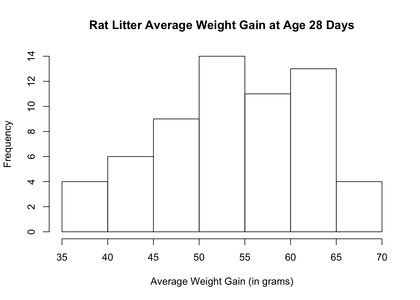

You can also do a boxplot to see if the average weight gain distribution is approximately normal.

boxplot(genotype$Wt, main = "Rat Litter Average Weight Gain at Age 28 Days",
     ylab = "Average Weight Gain (in grams)")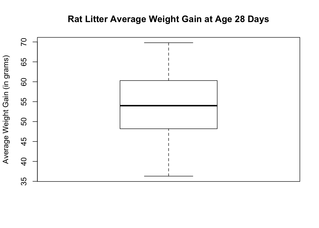

You can also check the normal quantile plot.

qqnorm(genotype$Wt, main = "Rat Litter Average Weight Gain at Age 28 Days",
     ylab = "Average Weight Gain (in grams)")
qqline(genotype$Wt)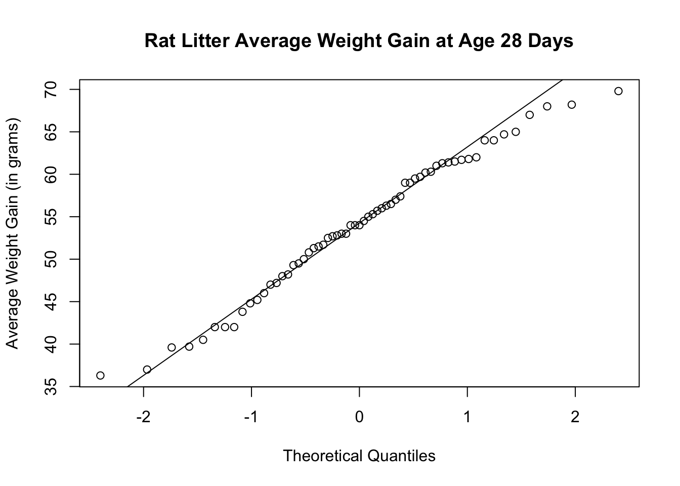

The histogram and boxplot show that the distribution is approximately symmetric with no visible outliers. The normal quantile plots lie approximately on a straight line. The distribution does not show any strong skewness and there are no visible outliers. We can conclude that the weight gain distribution is approximately normally distributed.

22.2 Two-Sided Hypothesis Test

To conduct a hypothesis test, we use the function, t.test( ). The arguments for t.test( ) may include the following unless required is specified:

quantitative variable (required)
mu = true Mean (required)
alternative = “two.sided”, “less”, or “greater”. If nothing is indicated, the argument defaults to two-sided.
conf.level = confidence level desired. If nothing is indicated, the argument defaults to 95% confidence level.

Let us do a hypothesis test to see if the weight gain of rat liters at 28 days is different from mu = 50 grams. This is a two-sided hypothesis test.

t.test(genotype$Wt, mu = 50)

## 
##  One Sample t-test
## 
## data:  genotype$Wt
## t = 3.7513, df = 60, p-value = 0.0003986
## alternative hypothesis: true mean is not equal to 50
## 95 percent confidence interval:
##  51.85334 56.08765
## sample estimates:
## mean of x 
##  53.97049

The t-test result shows a P-value of 0.0004, a 95% confidence interval of (51.85, 56.09) with a sample mean of 53.97 grams.

There are a lot of information given from the output of t.test( ). The R help page has a detailed list of what each object returned by the function contains. An alternative way to list the attributes is by using the function ls( ).

ls(t.test(genotype$Wt))

##  [1] "alternative" "conf.int"    "data.name"   "estimate"    "method"     
##  [6] "null.value"  "p.value"     "parameter"   "statistic"   "stderr"

We can now call out the specific attribute by appending the attribute at the end of the t.test( ) function.

# To calculate the confidence interval at 95% confidence level
t.test(genotype$Wt)$conf.int

## [1] 51.85334 56.08765
## attr(,"conf.level")
## [1] 0.95

# To calculate the degrees of freedom
t.test(genotype$Wt)$parameter

## df 
## 60

# To calculate the standard error
t.test(genotype$Wt)$stderr

## [1] 1.05842

# To calculate the test statistic be sure to include mu
t.test(genotype$Wt, mu = 50)$statistic

##        t 
## 3.751338

22.3 Calculating Confidence Interval

To calculate the confidence interval only, append $conf.int after the t.test( ) function. There is no need to enter mu as mu is not part of the confidence interval computation. If no confidence level is specified, R defaults to 95%.

# Calculates 95% confidence interval
t.test(genotype$Wt)$conf.int

## [1] 51.85334 56.08765
## attr(,"conf.level")
## [1] 0.95

# Calculates 92% confidence interval
t.test(genotype$Wt, conf.level = 0.92)$conf.int

## [1] 52.08561 55.85537
## attr(,"conf.level")
## [1] 0.92

From the results, we see that as the confidence level decreases, the confidence interval narrows.

22.4 One-Sided Hypothesis Test

To conduct a one-sided alternative hypothesis test and/or to compute a confidence level different from 95%, specify the alternative as “less” or “greater” and/or specify the confidence level using the argument, conf.level.

Suppose you conduct a one-sided hypothesis test with the alternative hypothesis greater than mu and the confidence level at 95%.

t.test(genotype$Wt, mu = 50, alternative = "greater")

## 
##  One Sample t-test
## 
## data:  genotype$Wt
## t = 3.7513, df = 60, p-value = 0.0001993
## alternative hypothesis: true mean is greater than 50
## 95 percent confidence interval:
##  52.20224      Inf
## sample estimates:
## mean of x 
##  53.97049

The result shows a P-value of 0.0002, alternative hypothesis of mu > 50, 95% confidence interval of (52.20, inf) and a sample mean of 53.97 grams.

Note that if you want to call out specific attributes of the one-sided alternative hypothesis, you will need to assign the t.test( ) function to an object.

Let us assign the t.test( ) function to an object called one_side.

one_side <- t.test(genotype$Wt, mu = 50, alternative = "greater")

We can now list and call out specific attributes of the new object.

# List attributes
ls(one_side)

##  [1] "alternative" "conf.int"    "data.name"   "estimate"    "method"     
##  [6] "null.value"  "p.value"     "parameter"   "statistic"   "stderr"

# Calculate sample mean
one_side$estimate

## mean of x 
##  53.97049

# See what alternative hypothesis was used
one_side$alternative

## [1] "greater"