Chapter 23 Inference on Two Independent Sample Means
We will use the dataset built into R called ToothGrowth which looks at the effect of Vitamin C on tooth growth in guinea pigs. The dataset shows the lengths of teeth after each guinea pig receives doses of vitamin C.
The variables of the dataset are:
- len which is the numeric tooth length measurement (unspecified units)
- supp which is the delivery method of Vitamin C - either by orange juice (OJ) or by ascorbic acid (VC)
- dose which is the dosage of the supplement - 0.5 ml/day, 1.0 ml/day or 2.0 ml/day
23.1 One-Sided Hypothesis Test
Suppose we want to see the effectiveness of the delivery method disregarding dosage. First, let us check assumptions before doing the hypothesis test: the two samples are independent and randomly selected from the population of interest and the sample size is greater than 30.
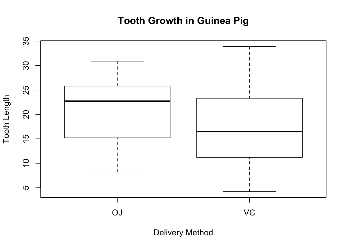
Let us check if there are any outliers by drawing the boxplot of the tooth length separated by the delivery method.
boxplot(ToothGrowth$len ~ ToothGrowth$supp,
        main = "Tooth Growth in Guinea Pig",
        xlab = "Delivery Method",
        ylab = "Tooth Length")
The boxplots do not show any visible outliers.
Before we do a hypothesis test, we need to split the dataset into subsets by delivery method. All data containing the OJ as supplement will be called oj and those with VC as supplement will be called vc.
# Orange juice as delivery method of Vitamin C
oj <- subset(ToothGrowth, supp == "OJ")
# Ascorbic acid as delivery method of Vitamin C
vc <- subset(ToothGrowth, supp == "VC")Additional arguments for t.test( ) may include the following:
- alternative = “two.sided”, “less”, or “greater”. If nothing is indicated, the argument defaults to two-sided.
- var.equal = TRUE or FALSE. TRUE means that the variances are equal and FALSE means the variances are unequal. This is a required argument.
- conf.level = confidence level desired. If nothing is indicated, the argument defaults to 95% confidence level.
For this example, we want to see if delivering vitamin C via orange juice enhances more tooth growth in guinea pigs than ascorbic acid. A one-sided hypothesis test will be conducted. Since we are not told whether the variances are equal or not, we will assume unequal variances to be on the conservative side. We will use the default, 95% confidence level.
##
##  Welch Two Sample t-test
##
## data:  oj$len and vc$len
## t = 1.9153, df = 55.309, p-value = 0.03032
## alternative hypothesis: true difference in means is greater than 0
## 95 percent confidence interval:
##  0.4682687       Inf
## sample estimates:
## mean of x mean of y
##  20.66333  16.96333
The result shows a t-statistic of 1.9153 with 55.3 degrees of freedom. The P-value is 0.03. The 95% confidence interval is (0.47, inf). From the result, delivery using orange juice seems to be statistically better than delivery via ascorbic acid for tooth growth in guinea pigs.
If you switch variables, use alternative = “less”.
##
##  Welch Two Sample t-test
##
## data:  vc$len and oj$len
## t = -1.9153, df = 55.309, p-value = 0.03032
## alternative hypothesis: true difference in means is less than 0
## 95 percent confidence interval:
##        -Inf -0.4682687
## sample estimates:
## mean of x mean of y
##  16.96333  20.66333
Both one-sided hypothesis show the same P-value and degrees of freedom. The t-statistic is negative of the other and the confidence interval goes in the other direction.
23.2 Two-Sided Hypothesis Test
Suppose we want to compare tooth growth between the two delivery methods at a dose of 2 ml/day. First, we subset the data as follows.
# Vitamin C delivery via orange juice at 2 ml/day
oj_two <- subset(ToothGrowth, ToothGrowth$supp == "OJ" & ToothGrowth$dose == "2")
oj_two
## len supp dose
## 51 25.5 OJ 2
## 52 26.4 OJ 2
## 53 22.4 OJ 2
## 54 24.5 OJ 2
## 55 24.8 OJ 2
## 56 30.9 OJ 2
## 57 26.4 OJ 2
## 58 27.3 OJ 2
## 59 29.4 OJ 2
## 60 23.0 OJ 2#Vitamin C delivery via ascorbic acid at 2 ml/day
vc_two <- subset(ToothGrowth, ToothGrowth$supp == "VC" & ToothGrowth$dose == "2")
vc_two## len supp dose
## 21 23.6 VC 2
## 22 18.5 VC 2
## 23 33.9 VC 2
## 24 25.5 VC 2
## 25 26.4 VC 2
## 26 32.5 VC 2
## 27 26.7 VC 2
## 28 21.5 VC 2
## 29 23.3 VC 2
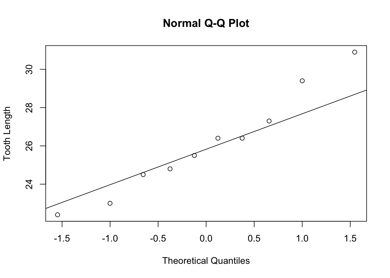
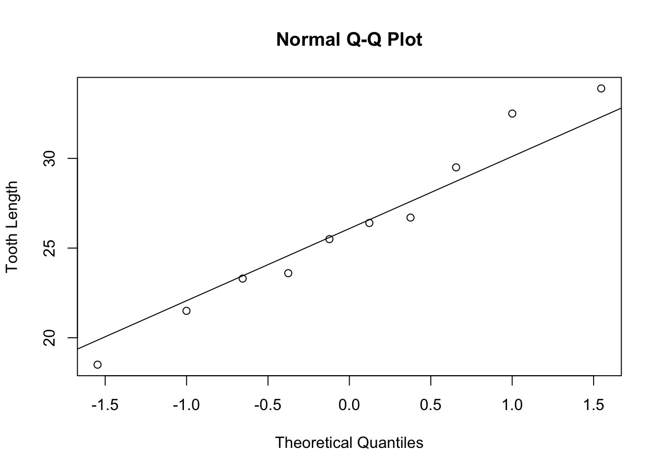
## 30 29.5 VC 2Note that the two subsets now have only 10 samples. It is important to check normality. We will do normal quantile plots to check for normality.


The normal quantile plots appear to be approximately normal with no visible outliers. We can now do a hypothesis test to check if there is any statistical difference in tooth growth using two different delivery methods at a dose of 2 ml/day.
Let us do a two-sided hypothesis test, with a confidence level of 90% using unequal variances.
##
##  Welch Two Sample t-test
##
## data:  oj_two$len and vc_two$len
## t = -0.046136, df = 14.04, p-value = 0.9639
## alternative hypothesis: true difference in means is not equal to 0
## 90 percent confidence interval:
##  -3.1335  2.9735
## sample estimates:
## mean of x mean of y
##     26.06     26.14
From the result, there does not seem to be any statistical difference in tooth growth for either supplement at 2 ml/day. P-value is extremely high (t-statistic almost 0) and the confidence interval includes 0.
23.3 Calculating Confidence Interval
To calculate the confidence interval only, append $conf.int after the t.test( ) function. There is no need to enter mu as mu is not part of the confidence interval computation. If no confidence level is specified, R defaults to 95%.
## [1] -3.79807  3.63807
## attr(,"conf.level")
## [1] 0.95
# To calculate 99% confidence level
t.test(oj_two$len, vc_two$len, var.equal = FALSE, conf.level = 0.99)$conf.int## [1] -5.239603 5.079603
## attr(,"conf.level")
## [1] 0.99