Chapter 20 Linear Regression Equation, Correlation Coefficient and Residuals

To determine the linear regression equation and calculate the correlation coefficient, we will use the dataset, Cars93, which is found in the package, MASS. Just like in previous example, we will only work with the variables, Weight, for weight of the car and MPG.city, for the miles per gallon achieved in driving around the city.

# Load package, MASS
library(MASS)

20.1 Linear Regression Equation

Let us revisit the scatterplot and best fit line of the weight of the car versus the miles per gallon achieved in the city from the dataset called Cars93.

plot(Cars93$Weight, Cars93$MPG.city,
     pch = 20,
     col = "blue",
     main = "Scatterplot of Weight of Car vs City MPG",
     xlab = "Weight of Car (in pounds)",
     ylab = "City Miles per Gallon")
abline(lm(Cars93$MPG.city ~ Cars93$Weight), col = "dark red")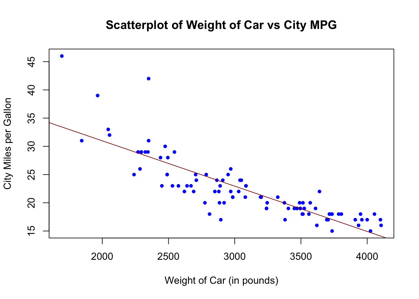

To find the equation for the regression line, we use the linear model function:
lm(response_variable ~ explanatory_variable)

lm(Cars93$MPG.city ~ Cars93$Weight)

## 
## Call:
## lm(formula = Cars93$MPG.city ~ Cars93$Weight)
## 
## Coefficients:
##   (Intercept)  Cars93$Weight  
##     47.048353      -0.008032

Under “Coefficients”, the “Intercept” is the y-intercept of the regression line and the other number is the slope. Therefore, the linear regression equation is:
City_Miles_per_Gallon = –0.008032*(Weight_of_Car) + 47.048353

20.2 Calculating Correlation Coefficient

Use the function cor(explanatory variable, response variable ) to calculate the correlation between the weight of the car and city miles per gallon.

cor(Cars93$Weight, Cars93$MPG.city)

## [1] -0.8431385

Since our regression line is sloping down, the correlation coefficient is negative.

20.3 Residual Plots

Recall that the residual data of the linear regression is the difference between the y-variable of the observed data and those of the predicted data. To plot the residuals:

First, figure out the linear model using the function, lm(response_variable ~ explanatory_variable). Assign the lm( ) function to an object.
Then use the function, resid(linear_model) to calculate the residuals. Assign the resid( ) function to an object.
To plot the residuals, we use the function, plot(explanatory_variable, residual).

Let us take a look at how to plot the residuals for our regression line that relates weight of the car versus city miles per gallon.

# Linear model assigned to the vector called Cars93_lm
Cars93_lm <- lm(Cars93$MPG.city ~ Cars93$Weight)
# Residual assigned to the vector called Cars93_res
Cars93_res <- resid(Cars93_lm)
# Plot Residuals
plot(Cars93$Weight, Cars93_res,
        main = "Residual Plot",
        xlab = "Weight of Car (in pounds)",
        ylab = "Residuals")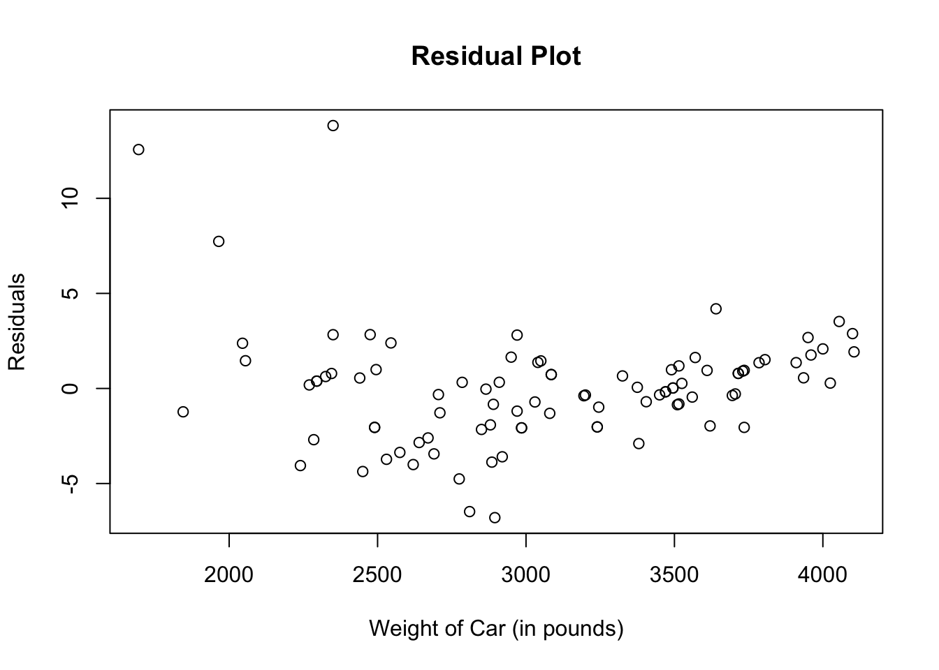

Sometimes a horizontal line through 0 is drawn to get a better visual of the residual plot. There are several different ways to draw the horizontal line. Any of the codes below will draw a horizontal line through 0.

abline(lm(residual, explanatory_variable)), which translates to lm(Cars93_res ~ Cars93$Weight) in our case
abline(y-intercept, slope), which translates to abline(0, 0) in our case
abline(h = horizontal_line), which translates to abline(h = 0) in our case

plot(Cars93$Weight, Cars93_res,
        main = "Residual Plot",
        xlab = "Weight of Car (in pounds)",
        ylab = "Residuals")
abline(lm(Cars93_res ~ Cars93$Weight))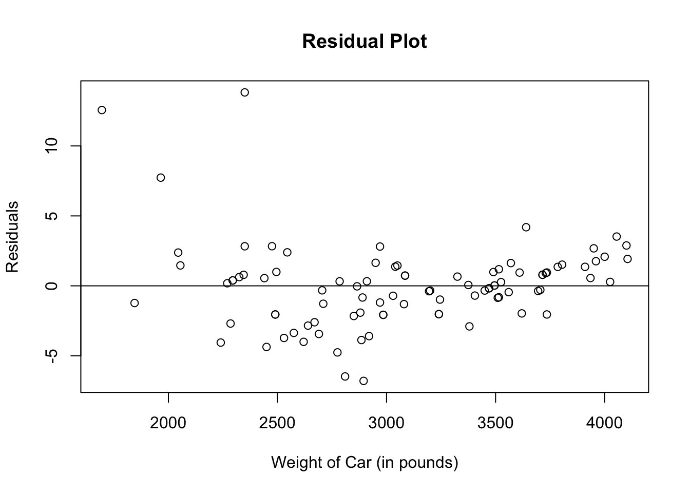

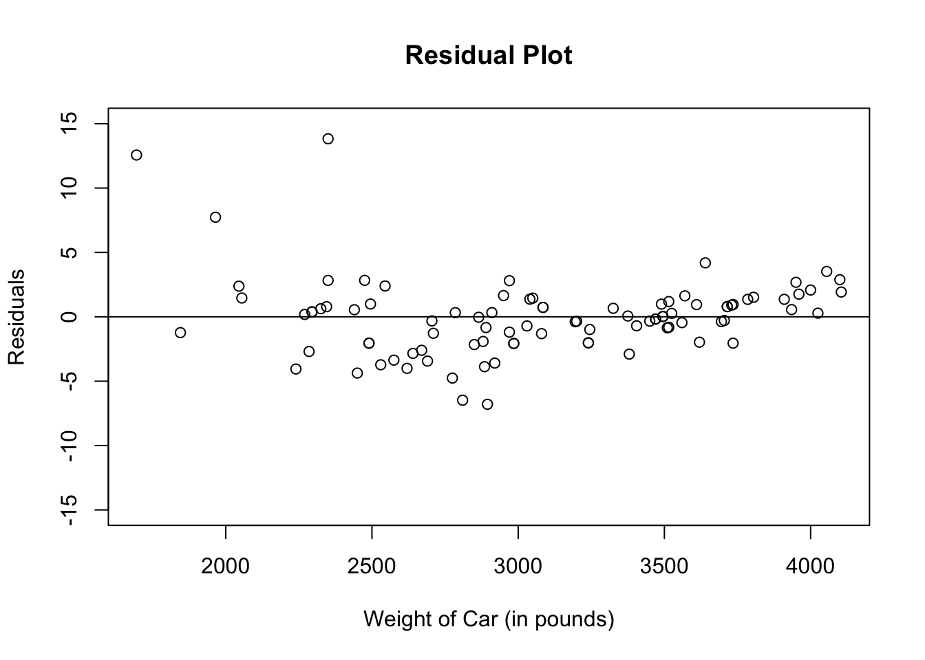
If you want the y-axis to be more proportional from 0, you can add the argument ylim to the plot( ) function and designate your lower and upper bounds for the y-axis.

plot(Cars93$Weight, Cars93_res,
     ylim = c(-15,15),
     main = "Residual Plot",
     xlab = "Weight of Car (in pounds)",
     ylab = "Residuals")
abline(lm(Cars93_res ~ Cars93$Weight))