Chapter 13 Some special designs
This chapter gives an introduction to some special randomized controlled trial designs. Cluster-randomized trials no longer randomize on individual (patient) level. Equivalence and non-inferiority trials differ from superiority trials in the sense that the objective of the trial is no longer to show that the intervention is better than control, but to show that two treatments are equivalent or one is non-inferior to the other one, respectively.
13.1 Cluster-randomized trials
Up to now, we have seen randomization of patients. Cluster-randomized trials allocate groups of patients en bloc to the same treatment.
Example 13.1 Kinmonth et al (1998) conducted an intervention study in primary care about whether additional training of nurses and general practitioners (GPs) in a general practice improves the care of patients with newly diagnosed type II diabetes mellitus. In this study, \(41\) practices were randomized to the status quo or to receive additional training for their staff.
13.1.1 Analysis
Standard methods can no longer be used, as patient responses from the same cluster are dependent. The intraclass correlation coefficient, i.e. the correlation between outcomes within a cluster, needs to be taken into account. In the following, we discuss two methods of analysis. First, we consider a simple approach, which consists of constructing a summary measure for each cluster and then analyze these summary values. Then, to analyse data on patient level, a mixed model formulation, a regression model with cluster-specific random effects, is needed. An alternative approach are so-called generalized estimating equations (GEEs). These methods will be applied to the following example:
Example 13.2 Oakeshott et al (1994), see also Kerry and Bland (1998a), report on the effect of guidelines for radiological referral on the referral practice of GPs where \(17\) practices in the intervention group received guidelines and 17 control practices were not sent anything. Outcome measure was the percentage of x-ray examinations requested that conformed to the guidelines. The data from the first 5 practices with and without intervention are shown below:
##          Group Practice Total Conforming Percentage
## 1 Intervention        1    20         20  100.00000
## 2 Intervention        2     7          7  100.00000
## 3 Intervention        3    16         15   93.75000
## 4 Intervention        4    31         28   90.32258
## 5 Intervention 5 20 18 90.00000## Group Practice Total Conforming Percentage
## 30 Control 30 21 14 66.66667
## 31 Control 31 126 83 65.87302
## 32 Control 32 22 14 63.63636
## 33 Control 33 34 21 61.76471
## 34 Control 34 10 4 40.00000Summary measure analysis
The analysis on practice level can be performed by applying a \(t\)-test to compare the percentage of x-ray examination in each practice. For simplicity we follow Kerry and Bland (1998a) and treat the percentages as a continuous outcome.
##
##  Two Sample t-test
##
## data:  Percentage by Group
## t = 1.8445, df = 32, p-value = 0.07438
## alternative hypothesis: true difference in means between group Intervention and group Control is not equal to 0
## 95 percent confidence interval:
##  -0.8310135 16.7625640
## sample estimates:
## mean in group Intervention      mean in group Control
## 81.52687 73.56109## [1] 7.965775The same results can be obtained with regression analysis, where we can also use the number of referrals as weight. The latter is the preferred analysis on practice level, as it takes into account the different cluster sizes (number of patients included per practice).
result <- lm(Percentage ~ Group, data = CRT)
result.w <- lm(Percentage ~ Group, data = CRT, weight = Total)
knitr::kable(tableRegression(result, xtable = FALSE))| Coefficient | 95%-confidence interval | \(p\)-value | |
|---|---|---|---|
| Intercept | 73.56 | from 67.34 to 79.78 | < 0.0001 |
| GroupIntervention | 7.97 | from -0.83 to 16.76 | 0.074 |
| Coefficient | 95%-confidence interval | \(p\)-value | |
|---|---|---|---|
| Intercept | 72.51 | from 68.30 to 76.72 | < 0.0001 |
| GroupIntervention | 6.98 | from 0.14 to 13.82 | 0.046 |
13.1.1.1 Logistic regression with random effects
The recommended analysis on patient level for a binary outcome is logistic regression with random effects for practices. The random effects account for possible correlation between patients treated in the same practice. We could in principle analyse the data in a long format, with a row for each patient and a binary outcome reflecting whether the x-ray from that particular patient conformed to the guidelines. However, as in standard logistic regression we can aggregate the data to binomial counts in each practice \(\times\) treatment group combination, but keep the random effects on practice level.
library(lme4)
CRT$Outcome <- cbind(CRT$Conforming, CRT$Total-CRT$Conforming)
result.glmm <- glmer(Outcome ~ Group + (1|Practice),
                     family = binomial, data = CRT)
(summary(result.glmm)$varcor)
## Groups Name Std.Dev.
## Practice (Intercept) 0.30862## Estimate Std. Error z value
## (Intercept) 1.0191021 0.1259360 8.092219
## GroupIntervention 0.4089998 0.1964084 2.082395
## Pr(>|z|)
## (Intercept) 5.858742e-16
## GroupIntervention 3.730643e-02## Effect 95% Confidence Interval P-value
## [1,] 1.505 from 1.024 to 2.212 0.037Just for illustration, we show an analysis of Example 13.2 on patient level where we ignore the clustering and aggregate the data to a 2x2 table (not recommended).
## aggregate data to 2x2 table ignoring cluster membership
Sums <- lapply(split(CRT, CRT$Group),
               function(x) c(Sums = colSums(x[,3:4]))
               )
Total <- c(Sums$Intervention["Sums.Total"], Sums$Control["Sums.Total"])
Conf <- c(Sums$Intervention["Sums.Conforming"],
          Sums$Control["Sums.Conforming"])
notConf <- Total-Conf
Group <- factor(c("Intervention", "Control"),
                levels = c("Intervention", "Control")
                )
tab <- xtabs(cbind(Conf, notConf) ~ Group)
print(tab)
##
## Group Conf notConf
## Intervention 341 88
## Control 509 193## 2 by 2 table analysis:
## ------------------------------------------------------
## Outcome : Conf
## Comparing : Intervention vs. Control
##
## Conf notConf P(Conf) 95% conf. interval
## Intervention 341 88 0.7949 0.7540 0.8305
## Control 509 193 0.7251 0.6908 0.7568
##
## 95% conf. interval
## Relative Risk: 1.0963 1.0260 1.1713
## Sample Odds Ratio: 1.4693 1.1027 1.9577
## Conditional MLE Odds Ratio: 1.4688 1.0935 1.9828
## Probability difference: 0.0698 0.0182 0.1191
##
## Exact P-value: 0.0087
## Asymptotic P-value: 0.0086
## ------------------------------------------------------This analysis is wrong, as it ignores the cluster structure and acts as if patients had been randomly assigned to treatment groups. This results in confidence intervals which are too narrow and \(P\)-values which are too small.
Mixed model for continuous outcomes
The mixed model formulation for a continuous outcome \(X_{ij}\) from patient \(j\) in cluster \(i\) is
| Treatment | Model |
|---|---|
| A | \(X_{ij} = \alpha + \xi_i + \epsilon_{ij}\) |
| B | \(X_{ij} = \alpha + \Delta + \xi_i + \epsilon_{ij}\) |
where
- \(\Delta\) is the treatment effect of B vs. A,
- \(\xi_i\) is a cluster-specific random effect with variance \(\sigma_b^2\),
- the errors \(\epsilon_{ij}\) have variance \(\sigma_w^2\).
The total variance is then \(\mathop{\mathrm{Var}}(X_{ij}) = \sigma^2 = \sigma_b^2 + \sigma_w^2\) and
the intraclass/intracluster correlation coefficient is \(\rho= \sigma_b^2/\sigma^2\).
The analysis can be performed with lme4::lmer().
13.1.2 Sample size calculation
In addition to a standard sample size calculation, we need the average cluster size \(\bar n_c\) and the intraclass correlation \(\rho\). The total number of patients receiving each treatment should then be
\[\begin{equation*} n = \underbrace{\frac{ 2 \sigma^2 (u+v)^2}{ \Delta^2}}_{\scriptsize \mbox{standard RCT sample size}} \times \quad \underbrace{(1+ \rho(\bar n_c-1))}_{\scriptsize \mbox{design effect $D_{\mbox{eff}}$}}. \end{equation*}\]
For example, suppose \(\bar n_c=7\) and \(\rho=0.5\), then \(D_{\mbox{eff}} = 4\), so 4-times as many patients are needed than for a standard RCT on patient-level.
If the number of patients
\[n = \frac{ 2 \sigma^2 (u+v)^2}{ \Delta^2} \cdot D_{\mbox{eff}}\]
has been calculated, then the number of clusters \(N_c\) receiving each treatment is \(n/\bar n_c\). Alternatively, we could directly calculate
\[\begin{equation*} N_c = \frac{ 2 (\sigma_b^2 +\sigma_w^2/\bar n_c) (u+v)^2}{ \Delta^2}. \end{equation*}\]
13.2 Equivalence and non-inferiority trials
Up to now, we discussed superiority studies. The aim of equivalence trials is not to detect a difference, but to establish equivalence of the two treatments. An equivalence trial needs pre-specification of an interval of equivalence \(I=(-\delta, \delta)\) for the treatment difference. If \(\delta\) is only specified in one direction, then we have a non-inferiority trial with non-inferiority interval \(I=(-\infty, \delta)\) or \(I=(-\delta, \infty)\), depending on the context. Non-inferiority trials are based on one-sided hypothesis tests to check whether one group is almost as good (not much worse) than the other group.
The following scenarios highlight why non-inferiority and equivalence studies may be more appropriate than superiority studies in certain cases. One scenario is when the intervention being evaluated is expected to perform similarly to the standard of care with respect to the primary endpoint but offers potential advantages in secondary endpoints. These advantages could include fewer side effects, reduced production costs, more convenient formulations (e.g., tablets instead of infusions), fewer required doses, or improvements in quality of life. Another scenario involves studies assessing the bioequivalence of drugs that share the same active ingredient, such as different formulations of the same medication or generic alternatives.
Table 13.2 (second column) compares superiority to equivalence studies in terms of the underlying test hypotheses for the treatment effect \(\Delta\). The point null hypothesis in a superiority trial is “too narrow” to be proven. If a superiority trial shows a large \(P\)-value, then the only implication is that there is no evidence against \(H_0\). In contrast, equivalence studies specify an interval of equivalence (through an equivalence margin \(\delta\)) as a composite alternative hypothesis with its complement as the null hypothesis. This construction makes it possible to quantify the evidence for equivalence. Figure 13.1 illustrates the hypotheses of the different design types.
| Design | Hypotheses | Sample size |
|---|---|---|
| Superiority | \(H_0\): \(\Delta=0\) vs. \(H_1\): \(\Delta \neq 0\) | \(n = \frac{ 2 \sigma^2 (z_{1-\alpha/2}+z_{1-{\beta}})^2}{ \Delta^2}\) |
| Equivalence | \(H_0\): \(\left\lvert\Delta \right\rvert> \delta\) vs. \(H_1\): \(\left\lvert\Delta \right\rvert\leq \delta\) | \(n = \frac{2 \sigma^2(z_{1-\alpha}+z_{1-{\beta/2}})^2}{\delta^2}\) |
| Non-inferiority | \(H_0\): \(\Delta < -\delta\) vs. \(H_1\): \(\Delta \geq -\delta\) | \(n = \frac{2 \sigma^2(z_{1-\alpha}+z_{1-{\beta}})^2}{\delta^2}\) |
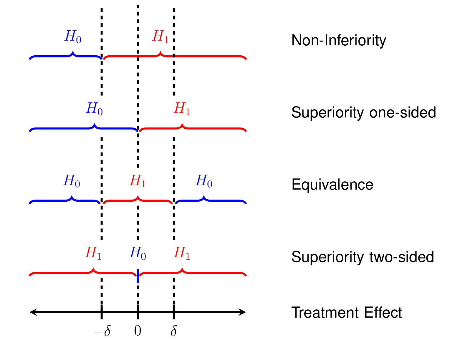
Figure 13.1: Comparison of superiority, equivalence, and non-inferiority study designs.
13.2.1 Equivalence trials
To assess equivalence, we compute a confidence interval at level \(\gamma\) for the difference in the treatment means. The treatments are considered equivalent if both ends of the confidence interval lie within the pre-specified interval of equivalence \(I=(-\delta, \delta)\). If this does not occur, then equivalence has not been established. The Type I error rate of this procedure is
\[\alpha \approx (1-\gamma)/2,\]
as shown in Appendix D.
For \(\gamma=90\%\), we have \(\alpha\approx 0.05\) and for \(\gamma=95\%\), we have \(\alpha\approx 0.025\).
The TOST procedure
An alternative approach to assess equivalence is the TOST procedure as follows:
- Apply Two separate standard One-Sided significance Tests
(TOST) at level \(\alpha\):
- Test 1 for \(H_0\): \(\Delta < - \delta\) vs. \(H_1\): \(\Delta \geq - \delta\)
- Test 2 for \(H_0\): \(\Delta > \delta\) vs. \(H_1\): \(\Delta \leq \delta\)
- If both one-sided tests can be rejected, we can conclude equivalence at level \(\alpha\).
Example 13.3 Remember Example 5.1 about a soporific drugs in terms of increase in hours of sleep compared to control. While this trial was not planned as an equivalence trial, let us suppose here the goal is to show equivalence at margin of \(\delta=0.5\) h. To make this scenario more reasonable, we simulate new (fake) data. Independent of the group (drug administered), we simulate all data from the same normal distribution with mean and variance estimated from the original data. You can see that there is less difference between the two groups in Figure 13.2 (fake data) than in Figure 5.3 (original data).
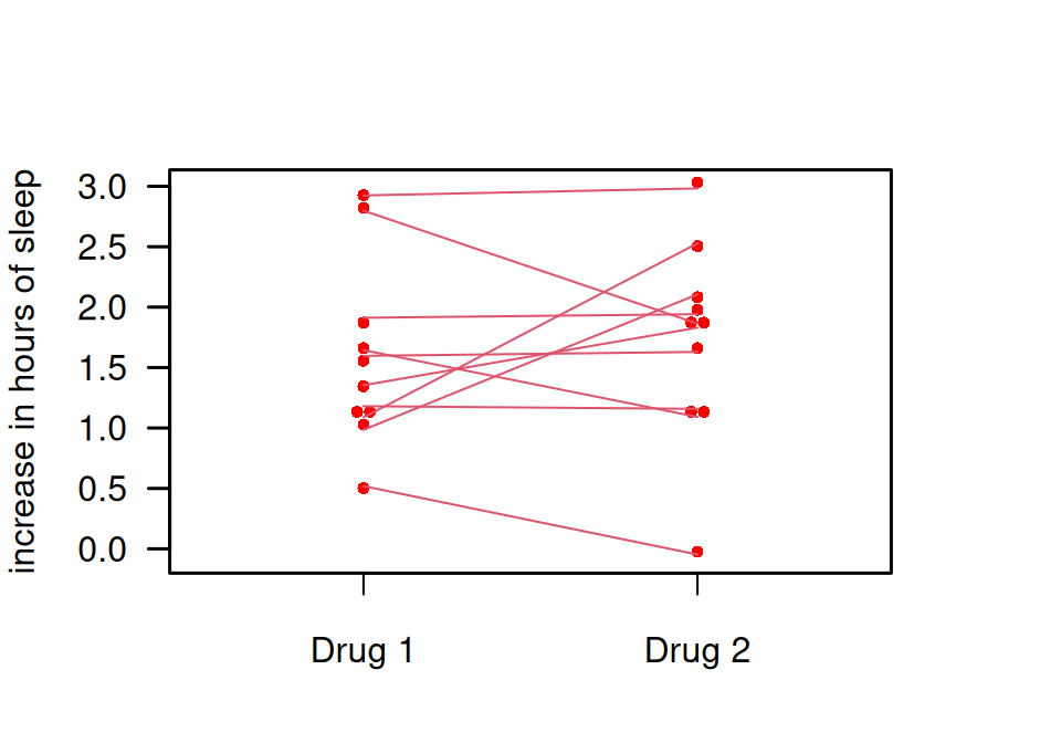
Figure 13.2: Comparison of two soporific drugs in a simulated (fake) example based on Example 5.1
## solution 1: confidence interval
extra1 <- sleep$extra[sleep$group==1]
extra2 <- sleep$extra[sleep$group==2]
res <- t.test(x=extra1, y=extra2, paired=TRUE, conf.level=0.9)
print(res$conf.int)
## [1] -0.5378899 0.3215748
## attr(,"conf.level")
## [1] 0.9The limits of the \(90\)% CI do not lie within the interval of equivalence (-0.5h, 0.5h). Hence, equivalence cannot be established.
## solution 2: TOST procedure
tost1 <- t.test(x=extra1, y=extra2, paired=TRUE, mu=-0.5,
                alternative="greater", sig.level=0.05)
print(tost1$p.value)
## [1] 0.06447987tost2 <- t.test(x=extra1, y=extra2, paired=TRUE, mu=0.5,
alternative="less", sig.level=0.05)
print(tost2$p.value)## [1] 0.01450592One \(P\)-value is larger than \(\alpha=5\%\), the other one is smaller. Hence, equivalence cannot be established.
Figure 13.3 shows different conclusions based on the confidence interval.
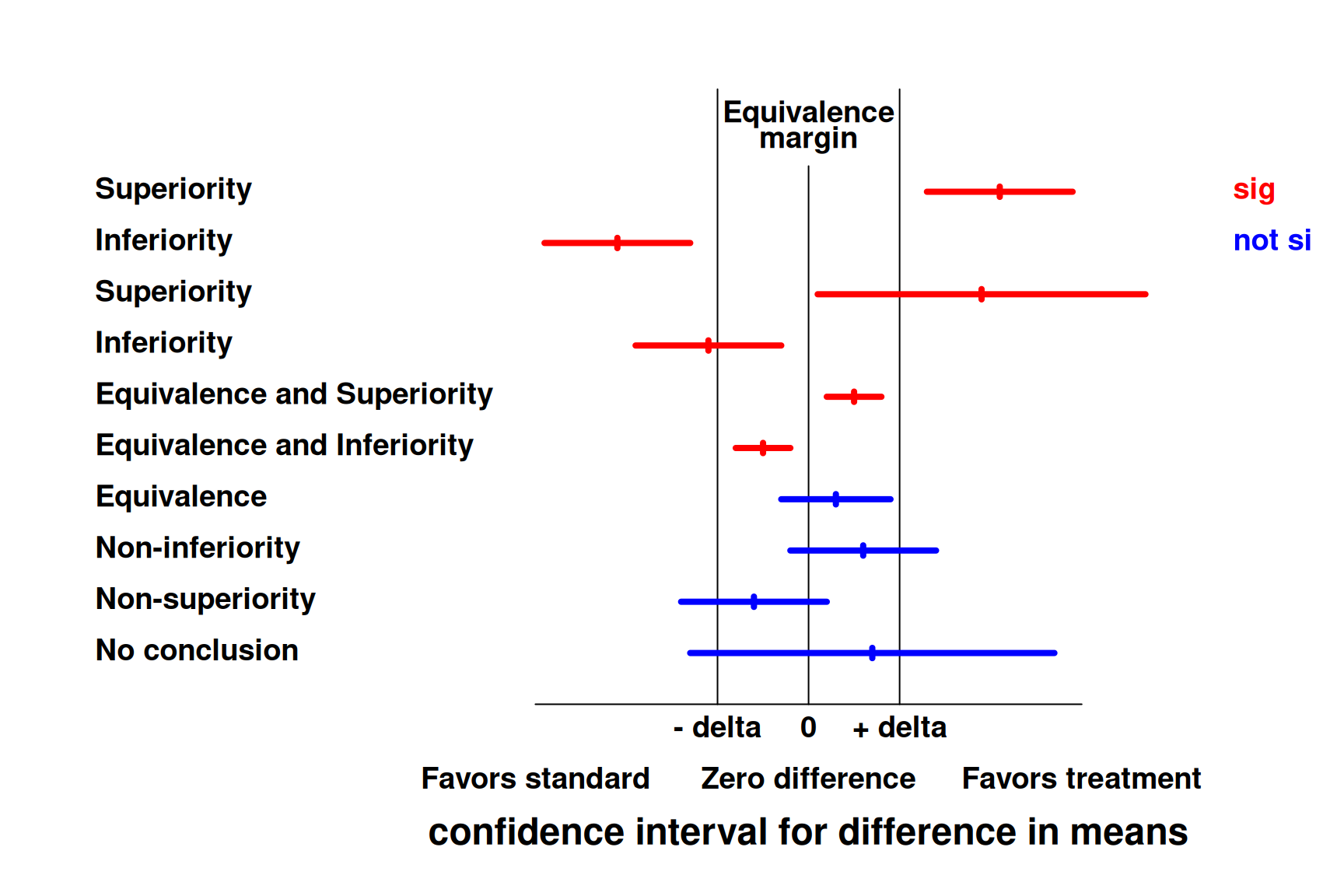
Figure 13.3: Concluding superiority, equivalence or non-inferiority based on a confidence interval for the difference in means.
Sample size calculation for continuous outcomes
Consider the hypotheses \(H_0: \left\lvert\Delta\right\rvert > \delta\) versus \(H_1: \left\lvert\Delta\right\rvert \leq \delta\). The Type I error rate is calculated for \(\Delta = \delta\). The power \(1-\beta\) is computed at the center \(\Delta=0\) of \(H_1\). Appendix D shows that the required sample size in each group then is:
\[\begin{eqnarray} n &=& \frac{2 \sigma^2(z_{\color{red}{(1+\gamma)/2}}+z_{\color{red}{1-{\beta/2}}})^2}{\delta^2} \\ & \approx & \frac{2 \sigma^2(z_{\color{red}{1-\alpha}}+z_{\color{red}{1-{\beta/2}}})^2}{\delta^2}, \tag{13.1} \end{eqnarray}\]
where \(z_{\gamma}\) is the \(\gamma\)-quantile of the standard normal distribution.
Table 13.2 (third column) compares the sample sizes of the different trial designs. The equivalence margin \(\delta\) takes over the role of the clinically relevant difference \(\Delta\). In practice, \(\delta\) is usually considerably smaller than \(\Delta\) in a related but conventional superiority trial. This typically leads to a larger sample size required for equivalence trials. Moreover, \(z_{1-\alpha}\) replaces \(z_{1 - \alpha/2}\) and \(z_{{1-{\beta/2}}}\) replaces \(z_{{1-{\beta}}}\). This is a consequence of the null hypothesis, but not the alternative, being two-sided in an equivalence trial.
Example 13.4 Holland et al (2017) conducted a randomized, controlled equivalence trial to assess whether home-based pulmonary rehabilitation was equivalent to center-based pulmonary rehabilitation. The primary outcome was the change in the 6 min walk distance test (6MWD). The paper states: “Sample size calculations indicated that 144 participants were required to be 80% sure that the 95% CI excluded a difference in the change in 6MWD of more than the equivalence limit of 25m, […], assuming an SD of 51m”.
n_equi <- function(delta, sd, alpha, beta){
  zalpha <- qnorm(1-alpha)
zbeta2 <- qnorm(1 - beta/2)
n <- 2*sd^2*(zalpha + zbeta2)^2/delta^2
return(n)
}

# ss per group with alpha = 2.5%
n <- n_equi(delta = 25, sd = 51, alpha = 0.025, beta = 0.2)
print(n)
## [1] 87.45538# ss per group with alpha = 5%
n2 <- n_equi(delta = 25, sd = 51, alpha = 0.05, beta = 0.2)
print(n2)## [1] 71.27861Using these values in Equation (13.1) with \(\alpha = 2.5\%\) gives \(n = 176 \neq 144\). The correct sample size is retrieved using \(\alpha = 5\%\), so one might wonder if they based their calculation on a 90% CI instead of a 95% CI.
13.2.2 Non-inferiority trials
Non-inferiority trials are useful if a proven active treatment exists and placebo-controls are not acceptable for ethical reasons. They are a special case of equivalence trials, but are conducted more often. To assess non-inferiority, just perform one of the two TOST tests, say
\[H_0: \Delta < - \delta \mbox{ vs. } H_1: \Delta \geq - \delta.\]
A one-sided superiority trial corresponds to \(\delta=0\). The alternative procedure based on confidence intervals computes a confidence interval at level \(\gamma\) and rejects \(H_0\) of inferiority if the upper bound is smaller than \(\delta\). The Type I error rate is \(\alpha = (1-\gamma)/2\).
The sample size (per group) is now
\[\begin{equation*} n = \frac{2 \sigma^2(z_{\color{red}{1-\alpha}}+z_{\color{red}{1-{\beta}}})^2}{\delta^2}. \end{equation*}\]
Sample sizes of the three designs are compared in Table 13.2 (third column). Table 13.3 compares the sample sizes for the three different designs of RCTs in practical examples assuming \(\Delta = \delta = \sigma = 1\) and different values for \(\alpha\) and \(\beta\). As before, the numbers can be adjusted for different values of \(\Delta/\sigma\) (respectively \(\delta/\sigma\)). For example, if \(\Delta/\sigma\) or \(\delta/\sigma = 1/2\) then the numbers have to be multiplied with 4.
| \(\alpha\) | \(\beta\) | Non-inferiority | Superiority | Equivalence |
|---|---|---|---|---|
| 5% | 20% | 12.4 | 15.7 | 17.1 |
| 5% | 10% | 17.1 | 21.0 | 21.6 |
| 2.5% | 20% | 15.7 | 19.0 | 21.0 |
| 2.5% | 10% | 21.0 | 24.8 | 26.0 |
Example 13.5 More than \(50\%\) of acute respiratory tract infections (ARTI) are being treated with antibiotics in primary care practice, despite mainly viral etiology. Procalcitonin (PCT) is a biomarker to diagnose bacterial infections. The PARTI trial (Briel et al, 2008) compares PCT-guided antibiotics use (decision depends on the value of the measured biomarker) versus standard of care. The hypothesis is that PCT-guided antibiotics are non-inferior to standard of care (non-inferiority trial).
The study cohort consists of 458 patients with ARTI. The primary endpoint was the number of days with restrictions due to ARTI. Patients were interviewed 14 days after randomization and the non-inferiority margin is \(\delta = 1\) day. Results showed that the mean increase in days with restriction with PCT-guided therapy was 0.14 , with 95% CI (from - 0.53 to 0.81 days) entirely below the margin \(\delta = 1\).
The main secondary endpoint was the proportion of antibiotics prescriptions where the PCT arm is hypothesized to be superior. The results were that 58/232 (25%) patients with PCT-guided therapy and 219/226 (97%) patients with standard therapy received antibiotics. This is a substantial reduction of antibiotics use with PCT-guided therapy of 72% (95% CI: 66% to 78%).
A more recent example of a non-inferiority trial is the study by Loeb et al (2022).
13.3 Additional references
Cluster-randomization is discussed in Bland (2015) (Sections 2.12, 10.13 and 18.8), equivalence and cluster-randomized trials in Matthews (2006) (Sections 11.5–11.6). The Statistics Notes Bland and Kerry (1997), Kerry and Bland (1998a), Kerry and Bland (1998b), Kerry and Bland (1998c) discuss different aspects of cluster-randomized trials. Studies where the special designs from this chapter are used in practice are for example Butler et al (2013), Burgess et al (2005), Lovell et al (2006).