Chapter 2 Continuous diagnostic tests
We now consider diagnostic tests that report a continuous test result.
2.1 Diagnostic accuracy measures
2.1.1 ROC curve
A threshold (“cut-off”) \(c\) can be used to dichotomize a continuous test result \(Y\) into positive (if \(Y \geq c\)) or negative (if \(Y < c\)). The sensitivity and specificity of continuous diagnostic tests depend on the threshold \(c\): \[\begin{eqnarray*} \mbox{Sens}(c) & = & \Pr(Y \geq c \,\vert\,D=1) \\ \mbox{Spec}(c) & = & \Pr(Y < c \,\vert\,D=0). \\ \end{eqnarray*}\]
Definition 2.1 The receiver operating characteristic curve (ROC curve) is a plot of \(\mbox{Sens}(c)\) versus \(1-\mbox{Spec}(c)\) for all possible thresholds \(c\). A useful test has a ROC curve above the diagonal, that is, \(\mbox{Sens}(c) + \mbox{Spec}(c) > 1\) for all thresholds \(c\).
Suppose we have data from a diagnostic test performed on \(n\) controls (that is, individuals without the disease in question) and \(m\) cases (individuals with the disease). If there are no ties, meaning that each observation has a unique value with no two observations being equal, the ROC curve is a step function with vertical jumps of size \(1/m\) and horizontal jumps of size \(1/n\). If several controls or cases have the same value, then the corresponding step size increases accordingly. If a case and a control have the same value then the ROC curve has a diagonal line segment. Furthermore, the ROC curve depends solely on the ranks of the data rather than the actual values. This means that the relative ordering of the data points is what influences the shape of the curve, not their specific magnitudes. As a result, any transformation that preserves the order of the data will not affect the ROC curve, making it scale-invariant.
Example 2.1 The gene expression data from a hypothetical study with \(n=23\) controls and \(m=30\) cases are shown in Figure 2.1. Table 2.1 gives sensitivity and specificity for selected cut-offs.
##    expr case
## 1 0.442    0
## 2 0.500    0
## 3 0.510    0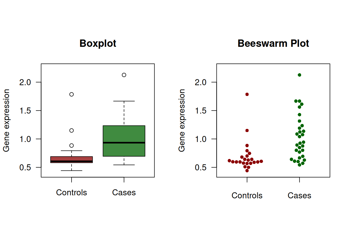
Figure 2.1: Continuous diagnostic test for gene expression.
| Cut-off | Sensitivity (in %) | Specificity (in %) |
|---|---|---|
| Inf | 0.0 | 100.0 |
| 2.13 | 3.3 | 100.0 |
| 1.78 | 3.3 | 95.7 |
| 1.19 | 30.0 | 95.7 |
| 0.88 | 56.7 | 87.0 |
| 0.67 | 80.0 | 69.6 |
| 0.57 | 93.3 | 21.7 |
| 0.51 | 100.0 | 8.7 |
| 0.50 | 100.0 | 4.3 |
| 0.44 | 100.0 | 0.0 |
Figure 2.2 then shows the standard ROC curve. The right plot gives a colorized version that indicates the corresponding cut-off value as indicated in the color scale on the right.
The following R code was used to produce Figure 2.2:
library(ROCR)
pred <- prediction(predictions = rocdata$expr,
                   labels = rocdata$case)
perf <- performance(pred, "tpr", "fpr")

par(mfrow = c(1, 2), pty = "s", las = 1)
plot(perf, xlab = "1-Specificity", ylab = "Sensitivity")
abline(0, 1, lty = 2)
plot(perf, colorize = TRUE,
     xlab = "1-Specificity",
     ylab = "Sensitivity")
abline(0, 1, lty = 2)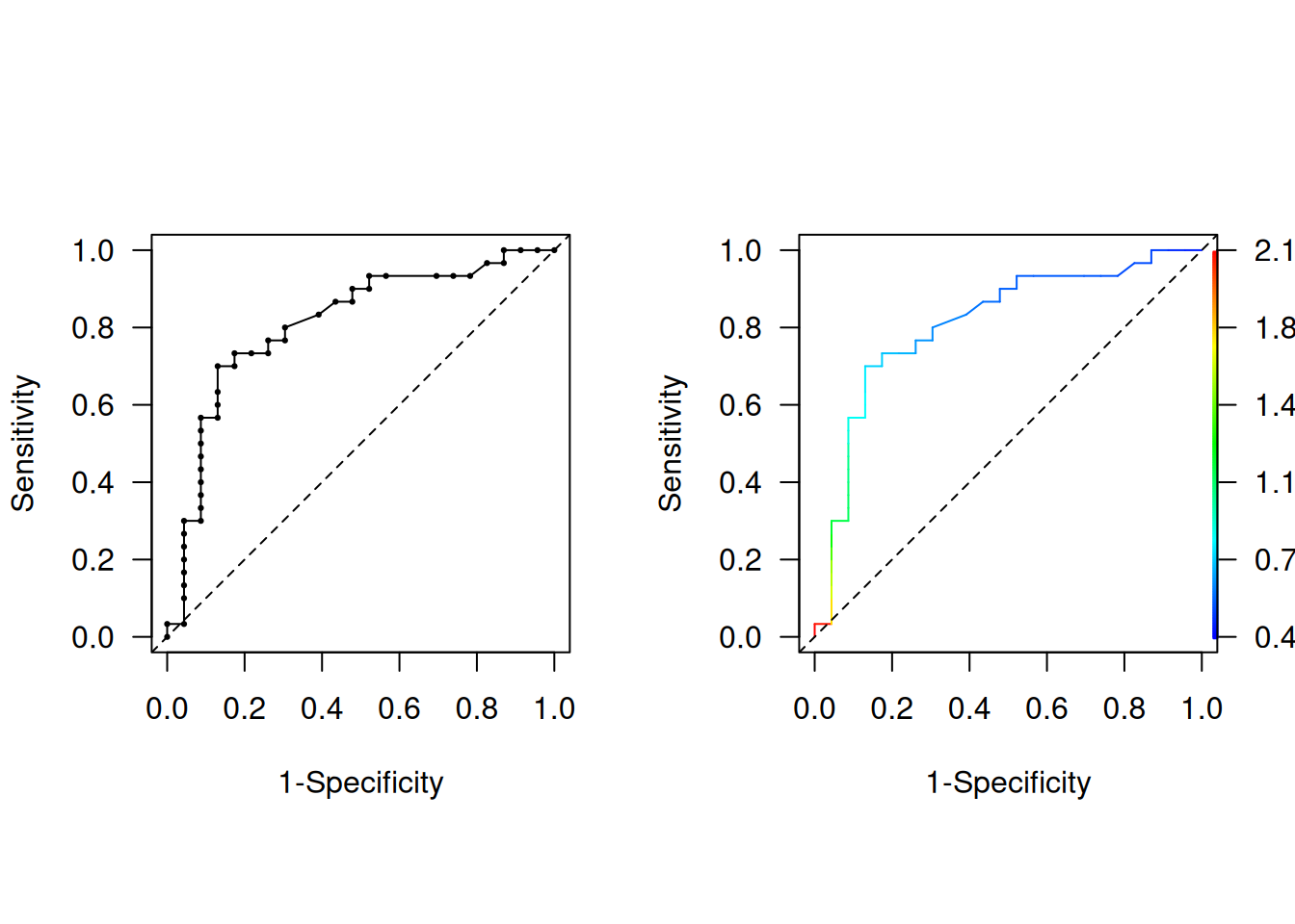
Figure 2.2: Empirical ROC curve, uncolorized (left) and colorized (right).
2.1.2 Area under the curve (AUC)
The most widely used summary measure to assess the performance of a classification model is the area under the ROC curve.
Definition 2.2 The area under the curve (AUC) is defined as
\[\begin{equation*} \mbox{AUC} = \int_0^1 \mbox{ROC}(t)dt. \end{equation*}\]
The AUC is interpreted as the probability that the test result \(Y_D\) from a randomly selected case is larger than the test result \(Y_{\bar D}\) from a randomly selected control:
\[ \mbox{AUC} = \Pr(Y_D > Y_{\bar D}). \]
A proof of this result can be found in Appendix C. Most tests have values between 0.5 (useless test) and 1.0 (perfect test).
The \(\mbox{AUC}\) can be conveniently computed based on the normalized Mann-Whitney U-Statistic:
cases <- rocdata[rocdata$case==1,]$expr
controls <- rocdata[rocdata$case==0,]$expr
ncases <- length(cases)
ncontrols <- length(controls)
n.pairs <- ncases*ncontrols
(auc <- wilcox.test(x=cases, y=controls)$statistic/n.pairs)
## W
## 0.8086957There is practical interest how to interpret a certain AUC value. Hond et al (2022) note that the variety in AUC labeling systems in the literature is substantial. However, some rough guidance may still be helpful for end-users, see Figure 2.3. Figure 2.4 illustrates how much two normal distributions (one for the cases and one for controls) with unit variance are apart for certain AUC values.
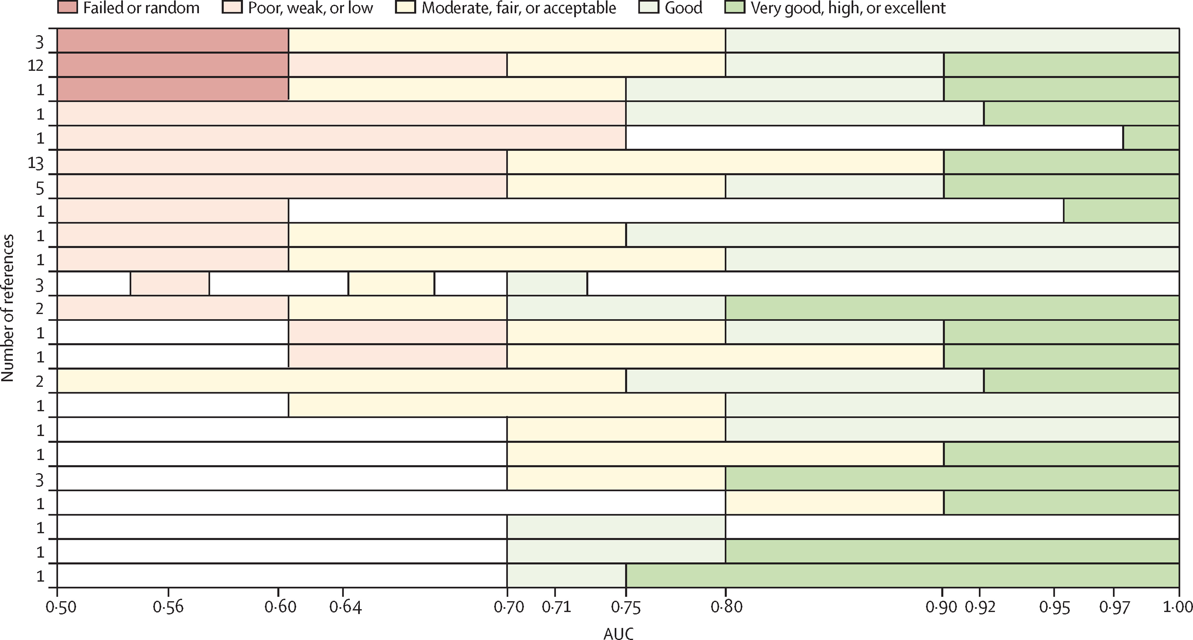
Figure 2.3: Different labelling systems of AUC from literature, taken from Hond et al (2022).
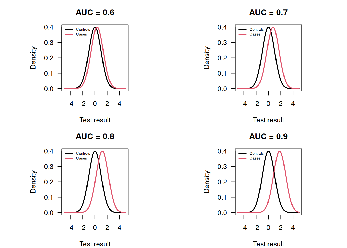
Figure 2.4: Normal distributions for cases and controls with unit variance and the corresponding AUC.
The standard error \(\mbox{se}({\mbox{AUC}})\) of the \({\mbox{AUC}}\) is difficult to compute and requires the execution of a computer program. The limits of a 95% Wald confidence interval for \({\mbox{AUC}}\) are: \[\begin{equation*} \mbox{AUC} - \mbox{ET}_{95} \mbox{ and } \mbox{AUC} + \mbox{ET}_{95}, \end{equation*}\] where the error term \(\mbox{ET}_{95} = 1.96 \cdot \mbox{se}({\mbox{AUC}})\).
Improved confidence intervals for \(\mbox{AUC}\) can be obtained with the logit transformation.
To avoid overshoot for diagnostic tests with high accuracy, we can use a Wald confidence interval for
\[\begin{eqnarray*}
\mathop{\mathrm{logit}}{\mbox{AUC}} &=& \log \frac{{\mbox{AUC}}}{{1-\mbox{AUC}}}. %%, \mbox{ with } \\[.3cm]
\end{eqnarray*}\]
The standard error of \(\mathop{\mathrm{logit}}{\mbox{AUC}}\) can be calculated with the Delta method.
The limits of the CI for \(\mathop{\mathrm{logit}}{\mbox{AUC}}\)
are back-transformed with
the inverse \(\mathop{\mathrm{logit}}\) function (“expit”).
A bootstrap confidence interval could also be used.
The Wald and logit Wald confidence intervals
can be computed using the function biostatUZH::confIntAUC()
and the boostrap confidence interval using pROC::ci.auc().
##         type     lower       AUC     upper
## 1       Wald 0.6843093 0.8086957 0.9330821
## 2 logit Wald 0.6541981 0.8086957 0.9042677
# bootstrap CI
library(pROC)
(ci.auc(response=rocdata$case,
predictor=rocdata$expr, method="bootstrap"))## Setting levels: control = 0, case = 1## Setting direction: controls < cases## 95% CI: 0.6782-0.9188 (2000 stratified bootstrap replicates)Example 2.2 The following simulated example illustrates overshoot, see Figure 2.5.
set.seed(12345)
groupsize <- 25
cases <- rnorm(n=groupsize, mean=3)
controls <- rnorm(n=groupsize, mean=0)
x <- c(cases, controls)
y <- c(rep("case", groupsize), rep("control", groupsize))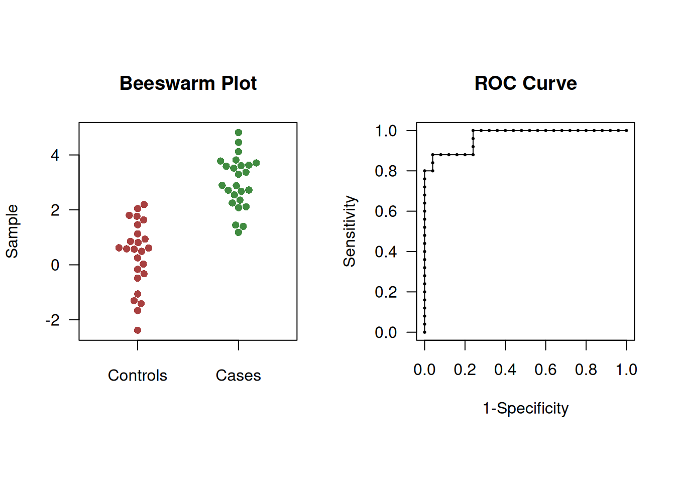
Figure 2.5: Beeswarm plot (left) and ROC curve (right) of simulated example to illustrate overshoot of confidence intervals.
In this case, the Wald CI overshoots whereas logit Wald and bootstrap CIs do not:
##         type     lower   AUC     upper
## 1       Wald 0.9290629 0.968 1.0069371
## 2 logit Wald 0.8959011 0.968 0.9906825
# bootstrap CI in library(pROC)
(ci.auc(response=y, predictor=x, method="bootstrap", conf.level = 0.95))## Setting levels: control = control, case = case## Setting direction: controls < cases## 95% CI: 0.9168-0.9968 (2000 stratified bootstrap replicates)2.1.3 Optimal cut-off
A simple method to derive a cut-off for a continuous diagnostic test is to maximize Youden’s index, see Equation (1.1). This cut-off corresponds to the point of the ROC curve that has maximal distance to the diagonal line.
Example 2.3 Jen et al (2020) conducted a study to assess the diagnostic performance of prostate-specific antigen (PSA) corrected for sojourn time. In order to maximize Youden’s index, a cut-off value of 2.5 ng/ml was chosen, for which the sensitivity was 75.3% and the specificity 85.2%.
However, this approach assumes equal importance for sensitivity and specificity and does not consider disease prevalence. The calculation of the optimal cut-off should account for the cost ratio \(\mbox{Cost(fp)}/\mbox{Cost(fn)}\) between false positives and false negatives, and take into account the prevalence (Pre) of the disease.
Definition 2.3 The minimize the overall cost, the optimal cut-off is where a straight line with slope
\[\begin{equation} b = \frac{1-\mbox{Pre}}{\mbox{Pre}} \times {\mbox{cost ratio}} \end{equation}\]
just touches the ROC curve.
To find the optimal cut-off, a straight line with slope \(b\) is moved from the top left corner of the ROC curve, where sensitivity and specificity are both equal to 1. The optimal cut-off is identified as the point where this line first intersects the ROC curve
Example 2.1 (continued) For example, if \(\mbox{Pre}=10\%\) and \(\mbox{Cost(fp)}/\mbox{Cost(fn)}=1/10\) in the gene expression data example, then \(b=9/10\) and the optimal cut-off is 0.8 as shown in Figure 2.6. This cut-off is also the optimal cut-off based on Youden’s Index, \(J = 0.70 + 0.87 - 1 = 0.57\).
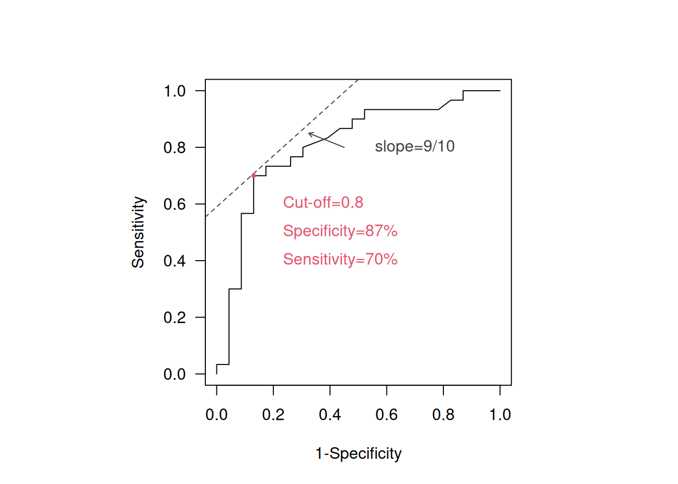
Figure 2.6: Identification of optimal cut-off in the ROC curve for 10% and Cost(fp)/Cost(fn)=1/10.
2.2 Comparing two continuous diagnostic tests
Suppose that \({\mbox{AUC}}(A)\) and \({\mbox{AUC}}(B)\) are available for two diagnostic tests \(A\) and \(B\) for the same disease. One way to compare their accuracy is to compute the difference in AUC: \[\Delta{\mbox{AUC}}={\mbox{AUC}}(A)-{\mbox{AUC}}(B).\] The standard error of \(\Delta{\mbox{AUC}}\) can be calculated using the formula
\[\begin{eqnarray*} {\mbox{se}}(\Delta {\mbox{AUC}}) &=& \sqrt{{\mbox{se}}({\mbox{AUC}}(A))^2 + {\mbox{se}}({\mbox{AUC}}(B))^2} \end{eqnarray*}\]
for unpaired samples.
For paired samples, a different formula based on
differences of placement values should be used.
The confidence interval for unpaired, respectively paired, samples
can be calculated using biostatUZH::confIntIndependentAUCDiff(),
respectively confIntIndependentAUCDiff().
Example 2.4 Figure 2.7 shows the ROC curve of two biomarkers for the diagnosis of pancreatic cancer (Wieand et al, 1989). A paired study design was used.
## [1] 141## y1 y2 d
## 1 28.0 13.3 0
## 2 15.5 11.1 0
## 3 8.2 16.7 0
## 4 3.4 12.6 0
## 5 17.3 7.4 0
## 6 15.2 5.5 0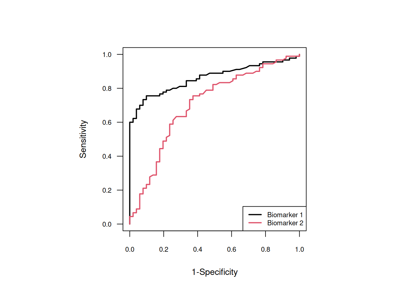
Figure 2.7: ROC curves of the two biomarkers.
The AUCs and \(\Delta{\mbox{AUC}}\) with 95% confidence intervals are:
case <- wiedat2b[,"d"]
y.cases <- wiedat2b[(case==1), c("y1","y2")]
y.controls <- wiedat2b[(case==0), c("y1","y2")]
(confIntPairedAUCDiff(y.cases, y.controls))
## outcome lower estimate upper
## 1 AUC Test 1 0.79001373 0.8614379 0.9112958
## 2 AUC Test 2 0.60637414 0.7055556 0.7884644
## 3 AUC Difference 0.04364262 0.1558824 0.2681221The confidence interval for the AUC difference does not include zero so there is evidence that Biomarker 1 has a better classification accuracy than Biomarker 2.
2.3 Additional references
Bland (2015) gives a gentle introduction to ROC curves in Chapter 20.6, see also the Statistics Note by Douglas G. Altman and Bland (1994). A comprehensive account of statistical aspects of ROC curves can be found in Pepe (2003) (Chapter 4 and 5). The methods from this chapter are used in practice, for example, in the following studies: Turck et al (2010), Cockayne et al (2011), Brown et al (2009), and Ikeda et al (2002).