Chapter 10 Subgroup analysis and multiple outcomes
Up to now we have focused on the comparison of two or more groups of patients, usually intervention vs. control. It is natural to investigate whether a treatment effect exists only in a certain subgroup of patients. Multiplicity issues arise if there are more than one subgroup-defining variable.
In addition, multiplicity issues also arise if more than one outcome are considered in a randomized trial. Here we describe methods that adjust the outcome-specific \(P\)-values and multivariate methods which combine the different outcomes in a single analysis.
10.1 Subgroup analysis
In a subgroup analysis, the objective is to determine whether the treatment effect is different for different types of patients. Possible subgroups are Male vs. Female, Children vs. Adults etc. Subgroups may also be disease-related, for example patients with/without diabetes or with/without a certain disease or disease status.
However, there are several problems which might arise. First, RCTs are usually powered to detect an overall difference between the two treatment groups. Analyses of subgroups will then have less power to detect a significant difference of the treatment effect between subgroups. Moreover, if subgroups are defined by many variables, the risk of a false positive (significant) finding increases. Finally, the choice of subgroups is difficult. Subgroup analyses are more credible if the subgroups were a priori specified (before the data were collected) rather than post hoc.
10.1.1 Comparing subgroups
Example 10.1 The Neonatal Hypocalcemia trial is a placebo-controlled trial of vitamin D supplementation of expectant mothers for the prevention of neonatal hypocalcemia (Cockburn et al, 1980). The primary endpoint is serum calcium level of the babies at 1 week of age. Table 10.1 shows the summary-level data for the serum calcium levels in the treatment and placebo groups. It shows it separately for the breast-fed and bottle-fed babies as the question is whether the treatment has a different effect in these two subgroups.
| Supplement | Placebo | Supplement | Placebo | |
|---|---|---|---|---|
| n | 64 | 102 | 169 | 285 |
| Mean | 2.445 | 2.408 | 2.3 | 2.195 |
| Var | 0.0853 | 0.0987 | 0.0752 | 0.1018 |
| SE | 0.0365 | 0.0311 | 0.0211 | 0.0189 |
## data
n <- c(64, 102, 169, 285)
mean <- c(2.445, 2.408, 2.300, 2.195)
var <- c(0.0853, 0.0987, 0.0752, 0.1018)
se <- sqrt(var/n)
Test for interaction
The correct approach to investigate whether there is a subgroup effect is a test for interaction. Suppose we have two subgroups defined by males (M) and females (F). To investigate if the treatment effect \(\theta\) differs between subgroups we consider the subgroup difference \[ \Delta \hat {\theta} = \hat \theta^{\tiny{\mbox{M}}} - \hat \theta^{\tiny{\mbox{F}}}, \] where \(\hat \theta^{\tiny{\mbox{M}}}\) and \(\hat \theta^{\tiny{\mbox{F}}}\) are the estimated treatment effects for males and females, respectively. Based on the standard error \[ \mbox{se}(\Delta \hat {\theta}) = \sqrt{\mbox{se}^2(\hat \theta^{\tiny{\mbox{M}}})+ \mbox{se}^2(\hat \theta^{\tiny{\mbox{F}}})}, \] tests and confidence intervals can be constructed.
The test for interaction is known in meta-analysis as the \(Q\)-test for heterogeneity and can also be used for more than two groups. Alternatively, a regression model with interaction between treatment and subgroup could be used, if individual-level data are available.
The test for interaction can be performed with the
function biostatUZH::printWaldCI().
Example 10.1 (continued) In the Neonatal Hypocalcemia trial, there is no evidence for a different treatment effect in the two subgroups (\(p=0.22\)). Perhaps the study sample size and specifically the breast-fed group (\(n=332\)) was too small to provide such evidence.
# Breast-fed babies:
se.breast <- sqrt(se[1]^2 + se[2]^2)

# Bottle-fed babies:
theta.bottle <- mean[3] - mean[4]
se.bottle <- sqrt(se[3]^2 + se[4]^2)


theta.diff <- theta.breast - theta.bottle
se.diff <- sqrt(se.breast^2 + se.bottle^2)
printWaldCI(theta.diff, se.diff)
## Effect 95% Confidence Interval P-value
## [1,] -0.068 from -0.177 to 0.041 0.22It is tempting to consider the treatment effect separately in each subgroup and to assess the existence of a treatment interaction based on an informal comparison of the \(P\)-values in each subgroup. As shown in Figure 10.1, for breast-fed and bottle-fed babies we obtain \(p=0.44\) and \(p=0.0002\), respectively, so one may argue that the two \(P\)-values are very different and conclude that there is a subgroup difference. However, this constitutes an erroneous and flawed reasoning. This becomes obvious in the following example: Suppose the effect estimates in the two groups are identical but the sample sizes are different such that one of the subgroups has a significant treatment effect whereas the treatment effect is non-significant in the other group. The difference in the \(P\)-values is then only a result of different sample sizes, without any difference in effect sizes. Indeed, with equal effect sizes in the two groups, the test for interaction will return a \(P\)-value of 1.0, so no evidence for a subgroup difference whatsoever. This example clearly illustrates that we need to compare effect sizes and not \(P\)-values to establish evidence for a difference between subgroups (Matthews and Altman, 1996).
##      Effect 95% Confidence Interval P-value
## [1,] 0.037 from -0.057 to 0.131 0.44## Effect 95% Confidence Interval P-value
## [1,] 0.105 from 0.049 to 0.161 0.0002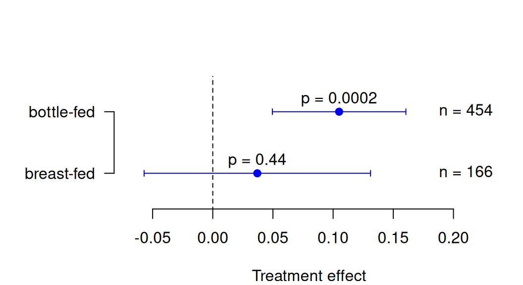
Figure 10.1: Treatment effects and \(P\)-values for each subgroup in the Neonatal Hypocalcemia Trial.
The test for interaction described above assumes normality of the effect estimates \(\hat \theta^{\tiny{\mbox{M}}}\) and \(\hat \theta^{\tiny{\mbox{F}}}\). If we have binary outcomes and want to compare relative risks or odds ratios, the test for interaction should be performed on the log scale because the distributions of log ratios tend to be closer to normal (Altman and Bland, 2003).
10.1.2 Selecting subgroups
The risk of false positive findings increases with increasing number of subgroup comparisons. For example, if we compare treatment effects in 20 different subgroups, then we would expect one of the analyses to yield a significant result (at \(\alpha=5\%\)), even if the treatment effect is the same in all subgroups (under the null hypothesis \(H_0\)). If the subgroups have been selected before the data were collected based on biological or clinical reasoning, then positive (significant) findings are more trustworthy than if subgroups have been defined post hoc.
10.1.3 Qualitative and quantitative interaction
The test for interaction tests the null hypothesis \(H_0\): \(\theta_1 = \theta_2 = \ldots = \theta_I\) of equal treatment effects \(\theta_i\) in \(i=1,\ldots,I\) subgroups. This is known as the \(Q\)-test in meta-analysis. A useful distinction between quantitative and qualitative interactions (subgroup differences) has been made.
Definition 10.1
- For a quantitative interaction, the size of the treatment effect \(\theta_i\) varies between subgroups \(i=1,\ldots,I\), but is always in the same direction.
- For a qualitative interaction, also the direction of the treatment effect varies between subgroups.
It has been argued that quantitative interactions are not surprising, whereas qualitative interactions are of greater clinical importance.
The method of Gail and Simon
The Gail-Simon test is a modified test for interaction with null hypothesis that there is no qualitative interaction (Gail and Simon, 1985), \[ H_0: \theta_i \geq 0 \mbox{ for all $i$ or } \theta_i \leq 0 \mbox{ for all $i=1,\ldots,I$.} \]
This test for qualitative interaction is based on the test statistic
\[\begin{equation*} T = \min\{Q^+,Q^{-}\}, \end{equation*}\]
where
\[\begin{eqnarray*} Q^+ = \sum_{i: \hat \theta_i \geq 0} Z_i^2 & \mbox{ and } & Q^- = \sum_{i: \hat \theta_i < 0} Z_i^2 \end{eqnarray*}\]
with \(Z_i=\hat \theta_i/\mbox{se}(\hat \theta_i)\) being the test statistics in each
subgroup \(i\). The reference distribution for \(T\) is non-standard,
so we use statistical software to calculate a \(P\)-value, as implemented in biostatUZH::gailSimon().
Example 10.2 In the National Surgical Adjuvant Breast and Bowel Project Trial (Fisher et al, 1983, sec. 9.2), the outcome was disease-free survival at 3 years, comparing chemotherapy (PF) only versus chemotherapy plus tamoxifen (PFT) for the treatment of Breast Cancer. The risk difference \(\theta\) is positive if disease free survival is more likely under PF. Four subgroups based on the progesterone receptor status (PR) and age are considered, see Table 10.2 and Figure 10.2.
| Metric | Age < 50 | Age >= 50 | Age < 50 | Age >= 50 |
|---|---|---|---|---|
| Risk difference \(\widehat{\theta}\) | 0.163 | -0.114 | -0.047 | -0.151 |
| \(\mbox{se}(\widehat{\theta})\) | 0.0788 | 0.0689 | 0.0614 | 0.0547 |
| \(\widehat{\theta}/\mbox{se}(\widehat{\theta})\) | 2.07 | -1.65 | -0.77 | -2.76 |
| \(P\)-value | 0.039 | 0.098 | 0.44 | 0.006 |
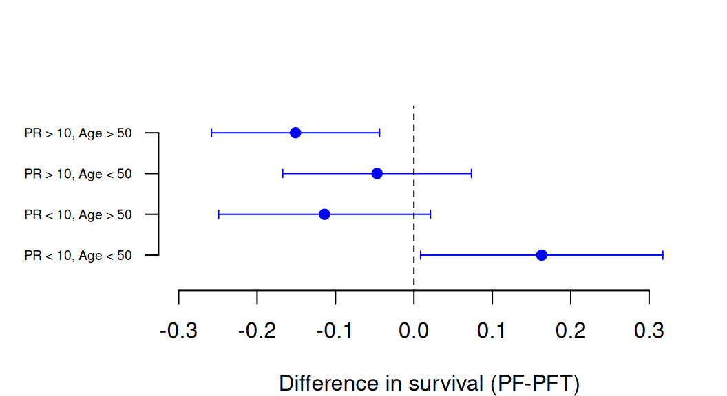
Figure 10.2: Treatment effects with confidence intervals for each subgroup in the National Surgical Adjuvant Breast and Bowel Project Trial.
The standard test for interaction gives \(p=0.0096\), as application of
the function meta::metagen() shows.
For the Gail-Simon test, we obtain
\(T=2.07^2=4.28\) and
\(p=0.088\).
So, there is moderate to strong evidence for a quantitative interaction,
but only weak evidence for a qualitative interaction.
## data
rd <- c(0.163, -0.114, -0.047, -0.151)
rd.se <- c(0.0788, 0.0689, 0.0614, 0.0547)

## Q-test for interaction
library(meta)
mymeta <- metagen(TE=rd, seTE=rd.se)
print(biostatUZH::formatPval(mymeta$pval.Q))
## [1] "0.01"## Gail and Simon test
pGS <- gailSimon(thetahat = rd, se = rd.se)
print(biostatUZH::formatPval(pGS[1]))## p-value
## "0.088"10.2 Multiple outcomes
Many clinical trials measure numerous outcome variables (primary and secondary) relevant to the condition studied. This raises multiplicity problems similar to those encountered when several subgroups are compared.
In what follows we assume that no distinction between primary and secondary outcomes has been made. In practice the problem of multiplicity is often avoided by selecting just one primary outcome. If there is more than one primary outcome, multiplicity adjustments need to be applied. Multiplicity adjustments can also be applied to secondary outcomes, but this is not always required (ICH Expert Working Group, 1999).
Example 10.3 Additionally to the primary endpoint (Epworth scale), the Didgeridoo Study (see Example 7.1) had also secondary endpoints:
- Pittsburgh quality of sleep index (range 0-21)
- Partner-rating of sleep disturbance (range 0-10)
- Apnoea-hypopnoea index (range 0-36)
Figure 10.3 shows the baseline and follow-up (4 months) measurements for the primary and secondary outcomes, compared between the treatment and control group. Change score analyses (using two-sample \(t\)-tests) have been performed for each of these outcomes, see Table 10.3 or also the published results (Puhan et al, 2005).
Puhan et al (2005) have selected the Epworth index as primary outcome, but in what follows we assume that no distinction between primary and secondary outcomes has been made.
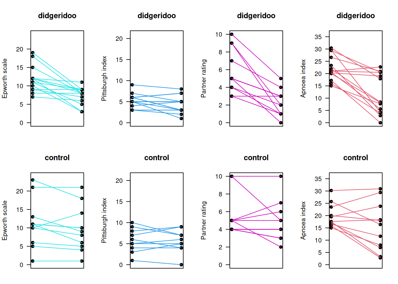
Figure 10.3: Baseline and follow-up measurements for primary and secondary outcomes in the Didgeridoo Study.
| Endpoint | Estimate | SE | t-value | p-value |
|---|---|---|---|---|
| Epworth scale | -3.0 | 1.3 | -2.3 | 0.03 |
| Pittsburgh index | -0.7 | 0.7 | -1.0 | 0.31 |
| Partner rating | -2.8 | 0.9 | -3.3 | 0.0035 |
| Apnoea index | -6.2 | 3.0 | -2.1 | 0.05 |
The next subsections explain two different approaches to prevent multiplicity problems: \(P\)-value adjustments and multivariate methods.
10.2.1 Adjusting for multiplicity
The problem with multiple outcomes is that the chance that at least one of them will provide a false significant result will be larger than the nominal \(\alpha\) level. Several adjustments for this are described in the following.
Definition 10.2 The family-wise error rate (FWER) is the probability of at least one false significant result. If \(k>1\) outcomes are considered, the FWER will be larger than the Type I error rate \(\alpha\). Under independence, we have
\[\begin{equation*} \mbox{FWER} = 1-(1-\alpha)^k. \end{equation*}\]
For small \(k\), the FWER under independence is close to the Bonferroni bound \(k \cdot \alpha\), which is an upper bound on the FWER obtained by applying the Bonferroni inequality, as shown in Figure 10.4.
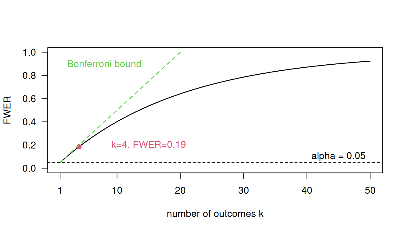
Figure 10.4: Family-wise error rate (FWER) under independence of the outcomes for a type I error rate \(\alpha = 0.05\) (black line) compared to the Bonferroni bound (green dotted line) as functions of the number of outcomes \(k\).
Bonferroni method
The Bonferroni method compares the \(P\)-values \(p_1, \ldots, p_k\), obtained from different outcomes, not with \(\alpha\), but with threshold \(\alpha/k\). If at least one of the \(P\)-values is smaller than \(\alpha/k\), then the trial result is considered significant at the \(\alpha\) level. This procedure controls FWER at level \(\alpha\). An equivalent procedure is to compare the adjusted \(P\)-values \(k \cdot p_i\) with the standard \(\alpha\) threshold.
Example 10.3 (continued) In the Didgeridoo Study, there is still evidence for a treatment effect after Bonferroni adjustments:
## [1] 0.03 0.31 0.0035 0.05## [1] 0.13 1.00 0.01 0.19However, the Bonferroni method is unsatisfactory as it takes only the smallest \(P\)-value into account, e.g.
- \(p=\) 0.01, 0.7, 0.8, 0.9 is “significant”,
- \(p=\) 0.03, 0.04, 0.05, 0.05 is “not significant”.
As a result, the Bonferroni method is very conservative and has low power.
Holm method
The Holm method is based on all ordered \(P\)-values \(p_{(1)} \leq \ldots \leq p_{(k)}\). A significant result is obtained if \[ k \cdot p_{(1)} \leq \alpha , \mbox{ or } (k-1) \cdot p_{(2)} \leq \alpha, \ldots \mbox{ or } p_{(k)} \leq \alpha. \]
Example 10.3 (continued) In the Didgeridoo study, there is also still evidence for a treatment effect after Holm adjustments, as one adjusted \(P\)-value is smaller than 0.05:
## [1] 0.10 0.31 0.01 0.10Simes’ method
Simes’ method (Simes, 1986) is also based on the ordered \(P\)-values \(p_{(1)} \leq \ldots \leq p_{(k)}\). A significant result is obtained, if \[ k \cdot p_{(1)} \leq \alpha, \mbox{ or } k/2 \cdot p_{(2)} \leq \alpha , \ldots \mbox{ or } p_{(k)} \leq \alpha. \]
Variations of it are the Hochberg (1988) and Hommel (1988) method.
Example 10.3 (continued) In the Didgeridoo study, there is also still evidence for a treatment effect after Simes adjustments (and its variants), as one adjusted \(P\)-value is smaller than 0.05:
## [1] 0.07 0.31 0.01 0.06## [1] 0.09 0.31 0.01 0.09## [1] 0.07 0.31 0.01 0.09Comparison of methods
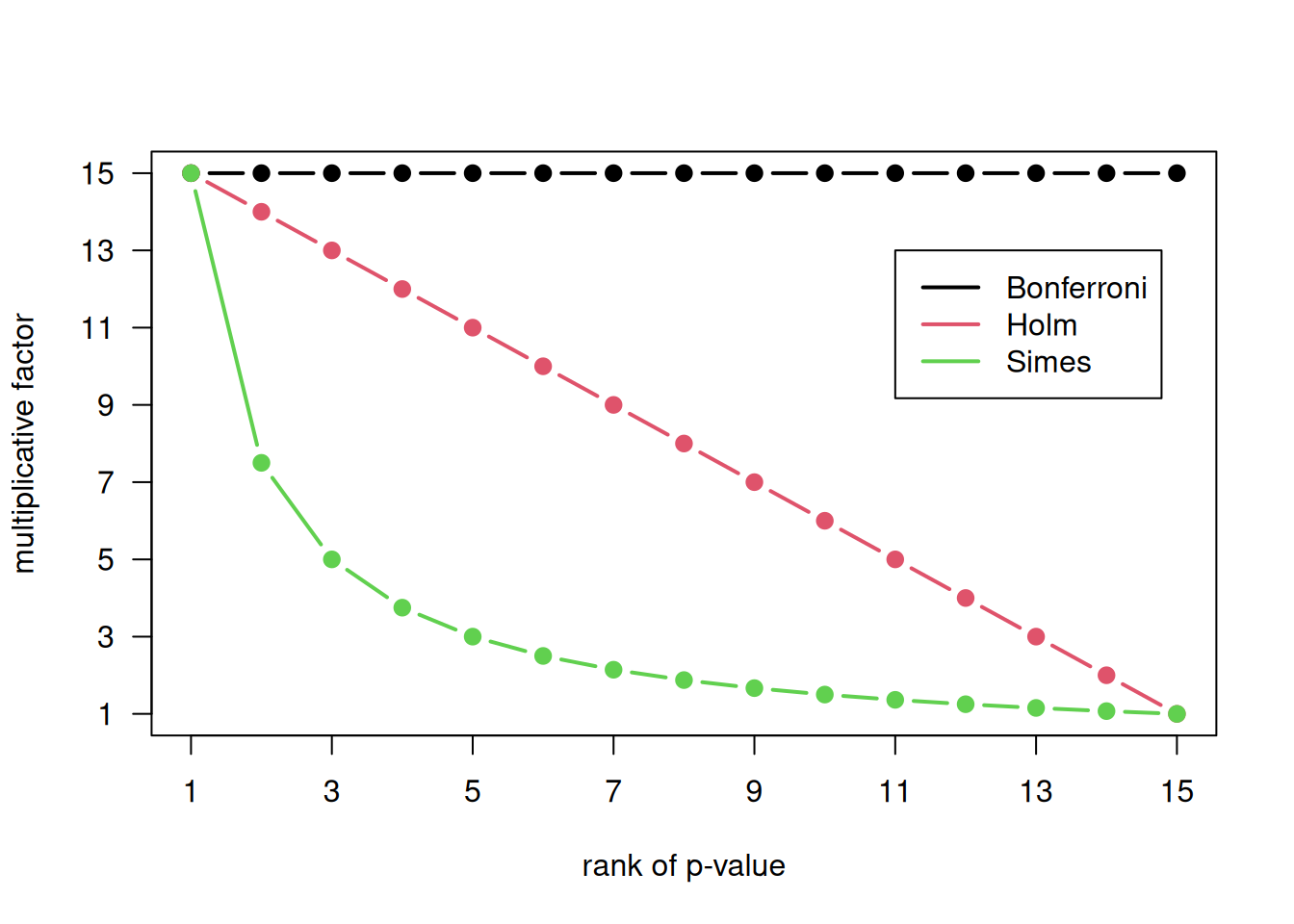
Figure 10.5: Multiplicative factors for multiplicity-adjustment of 15 \(P\)-values.
To obtain multiplicity-adjusted \(P\)-values, the ordinary \(P\)-values are multiplied with a factor, with subsequent truncation at 1 if necessary. The multiplicative factors for 15 \(P\)-values are compared in Figure 10.5 between the Bonferroni, Holm and Simes’ methods. Important differences between the three methods are the following:
- The Bonferroni method controls FWER, but has low power.
- The Holm method also controls FWER, but with a lower decrease of power than the classical Bonferroni method.
- If the \(P\)-values are independent or positively correlated, then Simes’ method also controls FWER. For positively correlated \(P\)-values, Simes’ method is even closer to the nominal \(\alpha\) level than the Holm method.
- Application of Holm and Simes requires knowledge of the \(P\)-value rank, whereas the Bonferroni method requires only knowledge of the number of \(P\)-values.
10.2.2 Multivariate methods
Multiplicity issues can also be avoided by considering the whole \(k\)-dimensional outcome vector simultaneously rather than separately.
Hotelling’s \(T\)-test
If all outcomes are continuous, then Hotelling’s \(T\)-test, a generalization of the \(t\)-Test, could be used. But this test accepts deviations from the null hypothesis in any direction, so typically lacks power.
Example 10.3 (continued) Hotelling’s \(T\)-test for the Didgeridoo study:
## Test stat:  16.226
## Numerator df:  4
## Denominator df:  18
## P-value:  0.02848
Combining outcomes in a summary score
Under the assumption that all outcomes are continuous and are orientated in the same direction, the following procedure can be used to combine multiple outcomes into one summary score:
- Standardize endpoints separately to a common scale: \[ \mbox{$z$-score} = {(\mbox{Observation} - \mbox{M})}/{\mbox{SD}}, \] where \(\mbox{M}\) and \({\mbox{SD}}\) are mean and standard deviation of the respective endpoint (ignoring group membership).
- Compute a summary score as the average of the different \(z\)-scores for each individual.
- Compare summary scores between treatment groups with a two-sample \(t\)-test.
Example 10.3 (continued) Figure 4 in Puhan et al (2005) shows the summary scores in the Didgeridoo study. Below we repeat the analysis. There are slight differences in the results, presumably due to a different handling of missing values (there was one patient with missing partner rating information and another one with missing Pittsburgh index measurement).
## z-scores
ep.z <- scale(alphorn$ep)
pi.z <- scale(alphorn$pi)
pa.z <- scale(alphorn$pa)
ap.z <- scale(alphorn$ap)

## summary scores
z.summary <- (ep.z + pi.z + pa.z + ap.z)/4

## t-test
print(summary.test <- t.test(z.summary ~ group, var.equal = TRUE))
##
## Two Sample t-test
##
## data: z.summary by group
## t = -3.228, df = 21, p-value = 0.004033
## alternative hypothesis: true difference in means between group 0 and group 1 is not equal to 0
## 95 percent confidence interval:
## -1.3205570 -0.2857226
## sample estimates:
## mean in group 0 mean in group 1
## -0.3829617 0.4201781## [1] -0.8031398O’Brien’s rank-based method
O’Brien’s rank-based method (O’Brien, 1984) is useful if some or all outcome variables are not normally distributed, such as non-normal continuous or categorical with a sufficiently large number of categories. The procedure starts by replacing each observation with its within-outcome rank. The test is accomplished by performing a \(t\)-test to compare the within-patient sums of ranks between the two treatment groups.
Example 10.3 (continued) O’Brien’s rank-based method in the Didgeridoo study:
## ranks and rank sums
ep.r <- rank(alphorn$ep, na.last="keep")
pi.r <- rank(alphorn$pi, na.last="keep")
pa.r <- rank(alphorn$pa, na.last="keep")
ap.r <- rank(alphorn$ap, na.last="keep")
rank.sum <- ep.r + pi.r + pa.r + ap.r

## t-test for rank sums
(obrian.test <- t.test(rank.sum ~ group, var.equal=TRUE))
##
## Two Sample t-test
##
## data: rank.sum by group
## t = -3.1392, df = 21, p-value = 0.004954
## alternative hypothesis: true difference in means between group 0 and group 1 is not equal to 0
## 95 percent confidence interval:
## -36.791720 -7.469818
## sample estimates:
## mean in group 0 mean in group 1
## 40.26923 62.40000## [1] -22.13077Figure 10.6 shows the within-outcome ranks for the primary outcome Epworth score and the within-patient sums of ranks for all outcomes. We can see a difference in the distribution with tendency for smaller ranks respectively rank sums in the Didgeridoo group. The \(t\)-test above identifies evidence for a difference in the mean rank sums (\(p=0.005\)), very similar to the \(P\)-value from the summary score analysis (\(p=0.004\)).
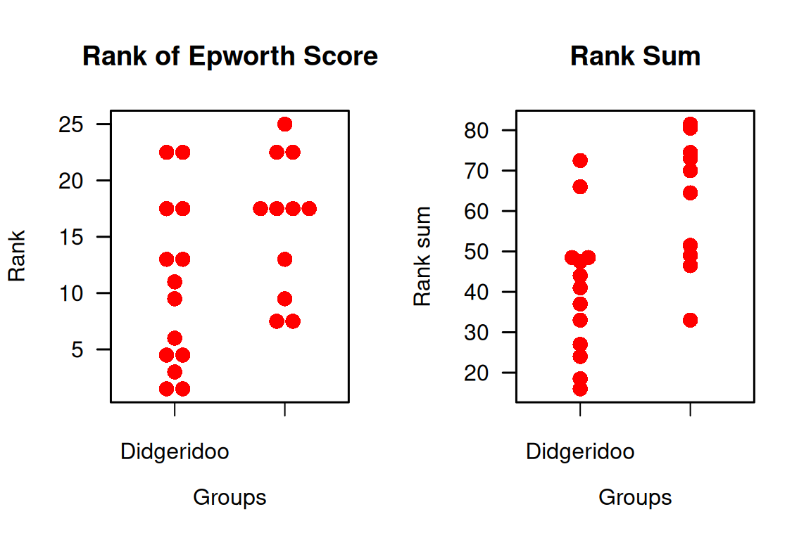
Figure 10.6: Ranks of the observations of the primary outcome in the Didgeridoo Study (left plot) and sum of the ranks of all outcomes (primary plus 3 secondary).
10.3 Additional references
The topics of this chapter are discussed in Bland (2015) (Ch. 9.10 Multiple Significance Tests) and Matthews (2006) (Ch. 9 Subgroups and Multiple Outcomes). Interactions are discussed in the Statistics Notes Matthews and Altman (1996) and Altman and Bland (2003).
More details on subgroup analyses in RCTs are given in Rothwell (2005). Studies where the methods from this chapter are used in practice are for example Pinkney et al (2013), Bennewith et al (2002) and de Fine Olivarius et al (2001).