Chapter 6 Randomization and allocation, blinding and placebos
In this chapter we discuss important techniques to allocate patients to two or more arms of an RCT. We also discuss blinding and placebos and close with the CONSORT reporting guidelines in Section 6.5.2.
6.1 Methods of allocation
There exist several methods to allocate patients to the different treatment groups in a clinical trial.
6.1.1 Simple randomization
Using simple randomization for allocation of \(2n\) patients to two treatment groups, A and B, the number of patients \(N_A\) in group A has a binomial distribution: \[ N_A \sim \mathop{\mathrm{Bin}}(2n, 1/2), \] which is the same for \(N_B\). However, one is fixed by the other: \(N_B = 2n - N_A\).
The distribution of the larger group size \(N_{\max}=\max(N_A,N_B)\) can then be derived as
\[ \Pr(N_{\max}=r) = \left\{ \begin{array}{rl} 2^{-2n} {2n \choose n} & \mbox{ for } r=n \\[.25cm] 2^{1-2n} {2n \choose r} & \mbox{ for } r=n+1,\ldots, 2n. \end{array} \right. \]
Proof. Given a specific \(N_A\), \(N_{\max}\) takes the following value:
| \(N_A\) | \(0\) | \(1\) | \(\dots\) | \(n - 1\) | \(n\) | \(n + 1\) | \(\dots\) | \(2n - 1\) | \(2n\) |
| \(N_B\) | \(2n\) | \(2n - 1\) | \(\dots\) | \(n + 1\) | \(n\) | \(n - 1\) | \(\dots\) | \(1\) | \(0\) |
| \(N_{\max}\) | \(2n\) | \(2n - 1\) | \(\dots\) | \(n + 1\) | \(n\) | \(n + 1\) | \(\dots\) | \(2n - 1\) | \(2n\) |
Equal sample size for both groups, \(r = n\), is a special case as it appears only once: \[\begin{equation*} \Pr(N_{\max} = n) = \Pr(N_A = n) = \binom{2n}{n} \left(\frac{1}{2}\right)^{2n} = 2^{-2n} \binom{2n}{n}. \end{equation*}\]
For \(r = n + 1, \dots, 2n\), the larger group can be either A or B, leading to: \[\begin{eqnarray*} \Pr(N_{\max} = r) & = & \Pr(N_A = r) + \Pr(N_A = 2n - r) \\ & = & \binom{2n}{r} \left(\frac{1}{2}\right)^{2n} + \binom{2n}{2n - r} \left(\frac{1}{2}\right)^{2n} \\ & \overset{\text{symm.}}{=} & 2 \cdot \binom{2n}{r} \left(\frac{1}{2}\right)^{2n} = 2^{1 -2n} \binom{2n}{r}. \end{eqnarray*}\]
For example, for \(n=15\), \(\Pr(N_{\max} \geq 20) = 0.10\). So, there is a substantial chance that the two groups will end up with markedly differing sizes, as illustrated in Figure 6.1. Unequal group sizes lead to a loss in power. For example, for Cohen’s \(d=1\), total sample size \(n_A+n_B=30\) and \(\alpha=0.05\), the loss in power is illustrated in Figure 6.2.
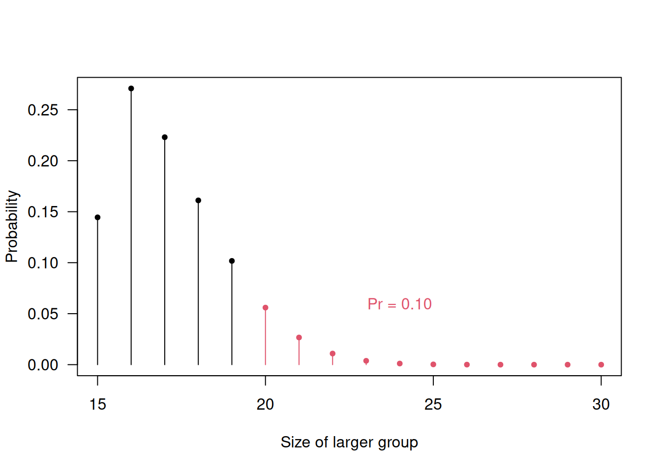
Figure 6.1: Probability for unequal group sizes with simple randomization and a total sample size of \(30\).
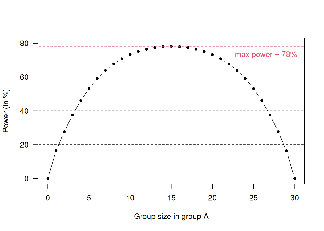
Figure 6.2: Loss in power for unequal group sizes in a scenario with \(d=1\), \(n_A+n_B = 30\) and \(\alpha = 0.05\).
6.1.2 Block randomization
The problem of unbalanced group sizes can be solved by using a form of restricted randomization with so-called random permuted blocks (RPBs). For example, with blocks of length 4, there are the following six different sequences of length 4 that comprise two As and two Bs:
| 1 | A | A | B | B |
| 2 | A | B | B | A |
| 3 | A | B | A | B |
| 4 | B | B | A | A |
| 5 | B | A | A | B |
| 6 | B | A | B | A |
In this case, the randomization selects randomly a block for every group of four patients. Block randomization using RPBs of length 4 ensures that group sizes never differ by more than 2. After every fourth patient, the two treatment groups must have the same size.
RPBs can also be used with other block lengths or for more than two groups, e.g. for a block length of 6 and three groups, there are 90 different sequences:| 1 | A | A | B | B | C | C |
| 2 | A | B | B | A | C | C |
| 3 | A | B | A | B | C | C |
| \(\vdots\) | \(\vdots\) | \(\vdots\) | \(\vdots\) | \(\vdots\) | \(\vdots\) | \(\vdots\) |
| 90 | C | C | B | B | A | A |
The following R code computes the different sequences for RPBs of length 4:
library(randomizeR)
## bc: length of block
## K: number of treatment groups
obj4 <- pbrPar(bc = 4, K = 2)
getAllSeq(obj4)
##
## Object of class "pbrSeq"
##
## design = PBR(4)
## bc = 4
## N = 4
## groups = A B
##
## The first 3 of 6 sequences of M:
##
## 1 B B A A
## 2 B A B A
## 3 A B B A
## ...Example 6.1 An RCT was conducted to examine the use of cold atmospheric plasma as a method to treat diabetic foot ulcers (Mirpour et al, 2020). The Methods section states that the patients were randomly assigned to the two treatment groups using block randomization with mixing block sizes of \(4\).
In some instances, the knowledge of the block length and of previous treatments allows the next treatment to be predicted. This may cause selection bias. RPBs with random block length have been suggested to avoid the potential for selection bias.
The following R code creates the randomization list for RBPs with random
block length of 2 and 4:
##
## Object of class "rRpbrSeq"
##
## design = RPBR(2,4)
## rb = 2 4
## filledBlock = FALSE
## seed = 1678498339
## N = 100
## K = 2
## ratio = 1 1
## groups = A B
##
## RandomizationSeqs BlockConst
## B A B A A B A B ... 4 4 2 2 4 ...## [1] "B" "A" "B" "A" "A" "B" "A" "B" "B" "A" "A" "B" "B"
## [14] "A" "A" "B" "A" "A" "B" "B" "B" "A" "B" "A" "B" "A"
## [27] "B" "A" "B" "A" "B" "A" "B" "A" "B" "A" "B" "A" "A"
## [40] "B" "A" "B" "A" "B" "B" "A" "A" "B" "B" "A" "A" "B"
## [53] "B" "B" "A" "A" "B" "B" "A" "A" "B" "A" "B" "B" "A"
## [66] "A" "A" "B" "B" "A" "B" "A" "B" "B" "A" "A" "A" "B"
## [79] "B" "A" "A" "B" "A" "B" "B" "A" "B" "A" "A" "B" "B"
## [92] "A" "A" "A" "B" "B" "A" "B" "B" "B"6.1.3 Unequal randomization
Unequal randomization can provide greater experience of a new treatment and may even encourage recruitment in certain trials. If the imbalance is no greater than 2:1, the loss in power is small (e.g. from 90% to 86% for \(\alpha=5\%\)). The treatment allocation sequences could be built by randomly selecting from the 15 blocks of length 6, comprising 4 As and 2 Bs.
The following R code computes the 2:1 allocation sequences
for a 2:1 allocation ratio using RPBs of length 6 for two groups:
library(randomizeR)
## bc: length of each block
obj <- pbrPar(bc=6, K = 2, ratio=c(2,1))
genSeq(obj, r=3, seed=123)
##
## Object of class "rPbrSeq"
##
## design = PBR(6)
## seed = 123
## N = 6
## ratio = 2 1
## groups = A B
## bc = 6
##
## The sequences M:
##
## 1 A B A A B A
## 2 B A A B A A
## 3 A B B A A A6.1.4 Stratification
Stratification is useful when there is imbalance with respect to prognostic factors. Suppose we wish to compare a new treatment \(T\) with placebo \(P\) to see if it improves a certain continuous outcome. An RCT is conducted with \(n\) patients in each group, all younger than 16 years of age. However, there is an important binary prognostic factor (e.g. age) which has level \(A\) (child, < 12 years) in a proportion of the eligible patients, otherwise it has level \(B\) (adolescent, \(\geq\) 12 years). Suppose that there is no treatment effect, but the mean outcomes \(\mu_A\) and \(\mu_B\) for type \(A\) and \(B\) differ: \(\mu_A \neq \mu_B\). Let us assume that we have conducted one particular trial with \(n\) patients per treatment group and
- \(n_T\) patients of type \(A\) (children) in group \(T\) and
- \(n_P\) patients of type \(A\) in group \(P\).
The expected outcome difference between group \(T\) and \(P\) then is
\[(n_T-n_P)(\mu_A-\mu_B)/n.\]
Although there is no treatment effect, this will be non-zero if \(n_T \neq n_P\). This bias is called allocation bias (see 4.2.2). Balance (\(n_T = n_P\)) can only be guaranteed on average across all possible trials, but not for our specific trial. Hence, the trial design should ensure that \(n_T \approx n_P\).
Stratification aims to control the imbalance between groups not with respect to their size, but with respect to their composition. The idea is to use different RPBs for different strata defined by relevant prognostic factors. For example, if age is an important prognostic factor, one may use an RPB design for children and another one for adults. The number of children (and of adults) receiving each treatment will then be very similar.
6.1.5 Minimization
If there are many prognostic factors, using a separate RPB for each possible combination of these factors becomes impractical. For example, if there are 5 binary prognostic factors, there will be already \(2^5=32\) strata. Minimization aims to balance the groups with respect to each factor, but not for each combination of the factors. The minimization algorithm is:
- Suppose a new patient enters the trial with certain values \(x_1, \ldots, x_J\) of relevant prognostic factors.
- The difference \(D_j\) of numbers of patients allocated to group \(A\) and patients allocated to group \(B\) is computed for the observed value \(x_j\) of each prognostic factor \(j=1,\ldots,J\).
- Compute the total difference \(D = \sum_j D_j\) and proceed as follows (with some \(p>1/2\)):
\[ \mbox{If} \left\{ \begin{array}{c} D = 0 \\ D < 0 \\ D > 0 \end{array} \right\} \begin{array}{c} \mbox{then allocate the new patient} \\ \mbox{to group A with probability} \end{array} \left\{ \begin{array}{c} 0.5 \\ p \\ 1-p \end{array} \right\}. \]
The minimization is deterministic if \(p = 1\) and \(D \neq 0\).
6.2 Blinding
Blinding is used to avoid assessment bias. We distinguish between single-blind and double-blind trials. In a single-blind trial the patient is unaware of the treatment being given, while in a double-blind trial, neither the doctor nor the patient knows what treatment is being given. In some trials, the statistical analysis is also carried out blinded because of subjective elements in any statistical analysis. For example, decisions like whether to transform the outcome variable, whether to compute risk differences, risk ratios or odds ratios for binary outcomes, or whether to include a covariate in the analysis all involve a degree of subjectivity. A precise statistical analysis plan helps in any case.
Example 6.1 (continued) In the RCT from Mirpour et al (2020), the patients were blinded, and the data were collected by a trained physician and nurse who were blinded to the randomization method and the treatment assignment. Moreover, the data were analyzed by a blinded investigator to the study groups.
6.3 Placebos
Placebos are treatments that look similar to the true treatment but contain no active ingredient. They have essentially two roles: first, placebos facilitate blindness in RCTs, as a treatment versus no treatment comparison cannot be blinded, but treatment versus placebo can often be blinded; second, placebos help control the placebo effect.
The placebo effect occurs if a patient exhibits a response to treatment, even though the treatment has no active component and cannot be having a direct effect. If only untreated controls (no treatment at all) are used, then we would not be able to tell whether an observed effect is due to treatment or to the placebo effect. Therefore, a placebo control group is usually selected to control the placebo effect. In some trials, both untreated and placebo control groups are used in addition to the usual intervention group to directly assess the size of the placebo effect.
6.3.1 The double-dummy technique
Placebos can also help in the comparison of two active treatments. Suppose a blue tablet is to be compared to a red tablet. Color cannot be changed, but the drug companies can produce placebo versions of the blue and red tablet, respectively. The double-dummy technique then gives both a blue and red tablet to each patient, in one group with blue active treatment and red placebo and vice versa in the other group. For example, this method is useful to blind a comparison of a treatment given as a tablet with an intravenous treatment.
6.4 ICH E10 guideline for control group
One major purpose of control groups is to discriminate the outcomes caused by treatment from the outcomes caused by other factors. The ICH E10 guideline describes in detail various types of control groups commonly employed to demonstrate efficacy, and for each considers the ability to minimize bias, ethical and practical issues associated with its use, usefulness and the quality of inference in particular situations, modifications of study design or combinations with other controls that can resolve ethical, practical, or inferential concerns, and overall advantages and disadvantages (see ICH (2000)).
Here we provide a high-level summary of E10 for control groups. We will show three types of most common control group.
The Placebo Control (P) helps us to analyse the treatment effect from ‘Response on standard-of-care (SoC) + Treatment’ vs ‘Response on SoC + Placebo’. This allows for blinding and randomization by requiring identical appearance or administration of treatment and placebo, but can have the risk of unblinding due to pharmacology. This approach is applicable in many situations, despite a lack of real-world applications, as it is very uncommon and not ethical to give placebo to patients in clinical practice.
The Active Control (A) is another possible control that also allows for blinding and randomization. It has ethical and practical advantages compared to Placebo Control. There are different possible trial objectives, for example showing superiority (new treatment is more effective than active control) or non-inferiority (new treatment is not less effective than active control), and more information can be found in Chapter 13. There are limitations, however, such as having more treatment exposure than control due to large sample sizes, and regional differences in SoC.
The External Control (E) uses data from patients in a previous trial as control, and a single arm trial is given. This is used in some particular settings, for example for serious diseases with high mortality, for rare diseases, for pediatric drug development, or when no other effective treatments are available. It has many challenges, including the loss of randomization and blinding, and the difficulty to ensure that current patients are comparable to earlier patients. Hybrid designs augment a concurrent control (P or A) arm with E data, to strengthen the overall control arm.
6.5 Reporting guidelines for clinical trials
6.5.1 The SPIRIT Statement
The SPIRIT (Standard Protocol Items: Recommendations for Interventional Trials) statement provides evidence-based recommendations for the minimum content of a clinical trial protocol (Chan et al, 2025; Hróbjartsson et al, 2025). SPIRIT is widely endorsed as an international standard for trial protocols. The recommendations are outlined in a 34-item checklist (see Figures 6.3 and 6.4), and figure (template of recommended content for the schedule of enrolment, interventions, and assessments). Important details for each checklist item can be found in the Explanation & Elaboration paper (Hróbjartsson et al, 2025). The items 19, 27a, 27b, 27c, and 27d are statistical, and are closely related to, i.e., need to correspond with, items 10, 12, 16, and 21a.
The current recommendations have been established in 2013 (Chan et al, 2013), and updated in 2025 (Chan et al, 2025) (see https://www.consort-spirit.org/).
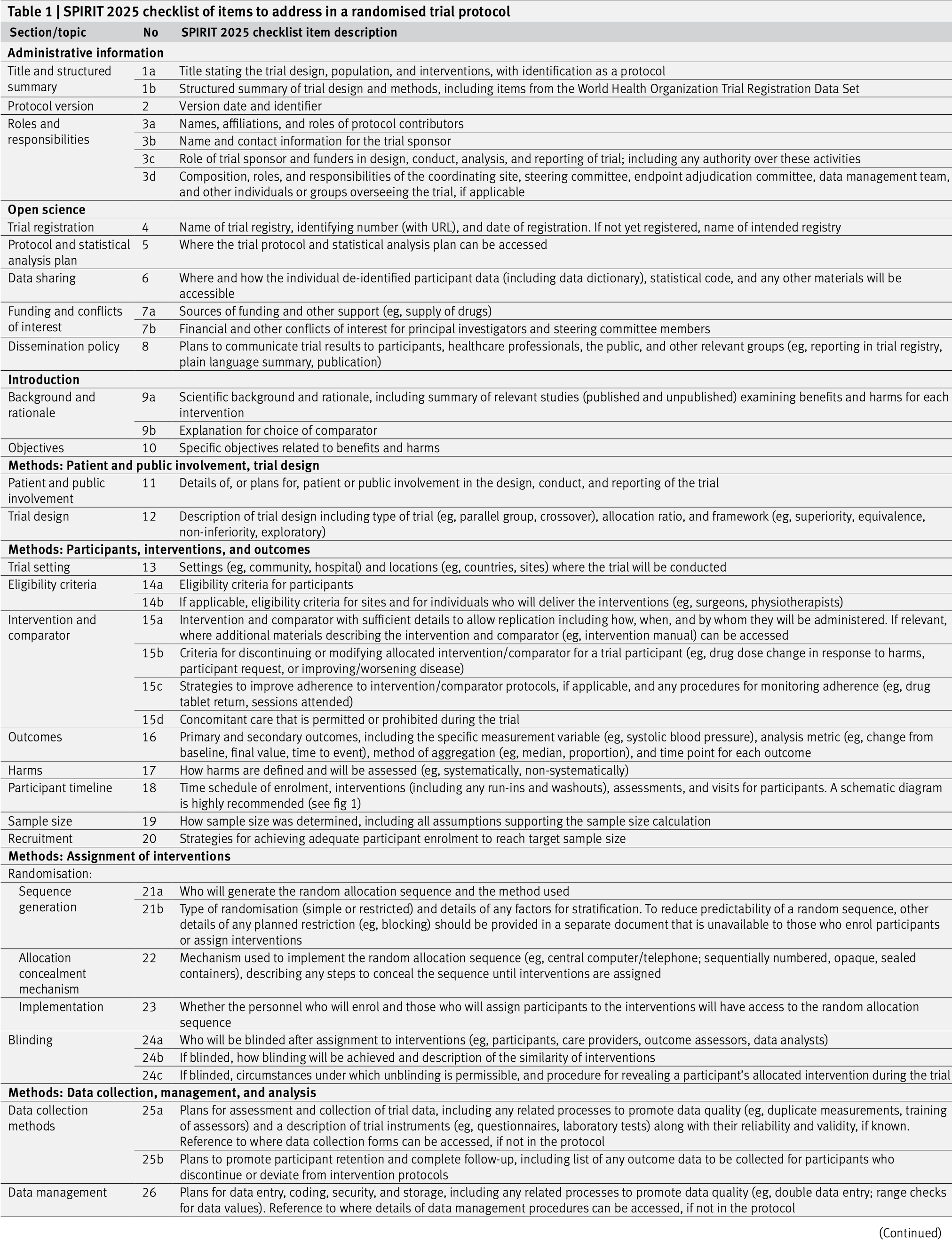
Figure 6.3: The SPIRIT checklist (items 1–26).
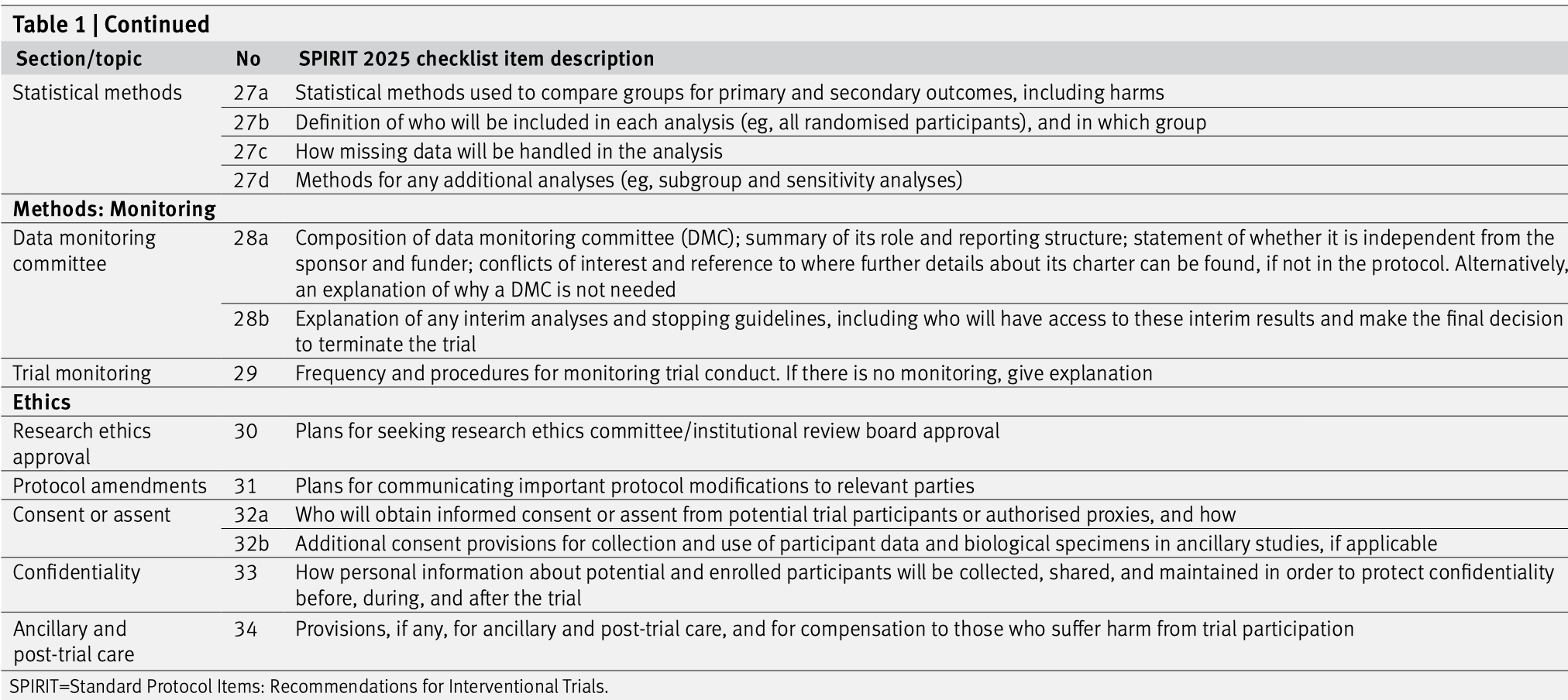
Figure 6.4: The SPIRIT checklist (items 27–34).
6.5.2 The CONSORT Statement
The CONSORT (CONSolidated Standards Of Reporting Trials) statement is an evidence-based minimum set of recommendations for reporting RCTs (Hopewell et al, 2025a, 2025b). It encompasses various initiatives developed by the CONSORT Group to alleviate the problems arising from inadequate reporting of RCTs. It offers a standard way for authors to prepare reports of trial design and analysis, facilitating their complete and transparent reporting, and aiding their critical appraisal and interpretation. The CONSORT Statement comprises a 30-item checklist, see Figure 6.5, and a flow diagram, see Figure 6.6.
The current recommendations have been established in 2010 (Schulz et al, 2010), and updated in 2025 (Hopewell et al, 2025a) (see https://www.consort-spirit.org/).
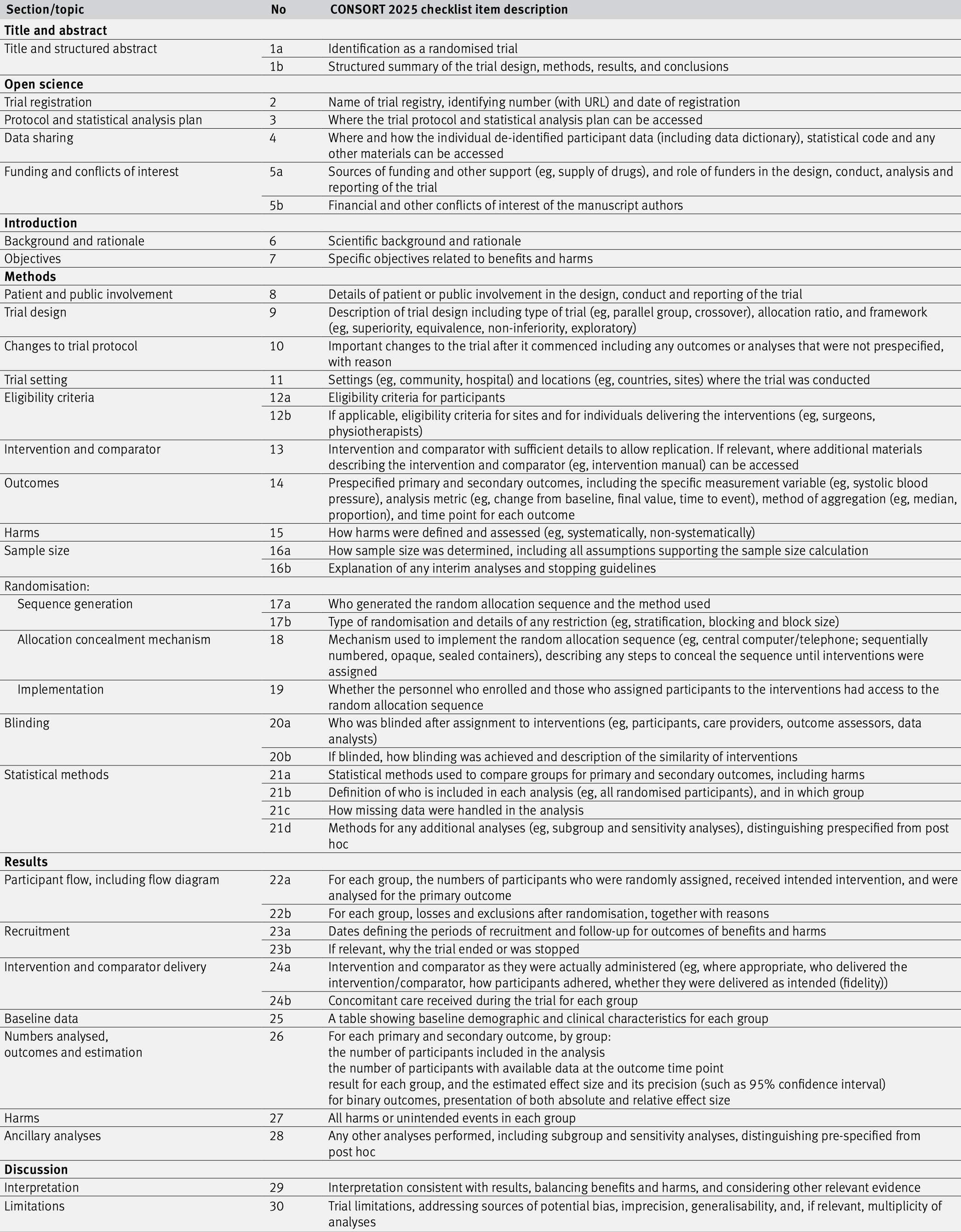
Figure 6.5: The CONSORT checklist.
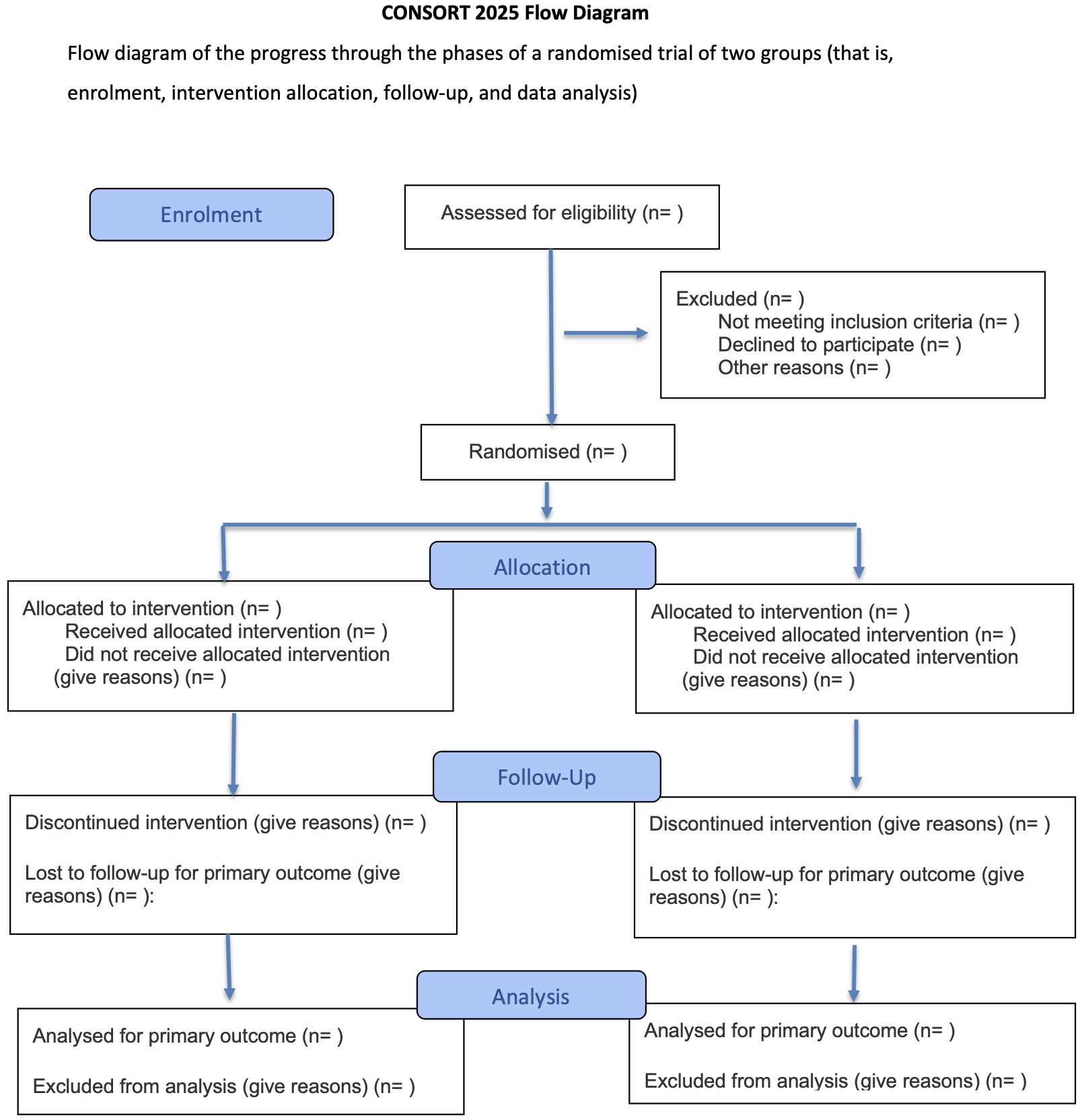
Figure 6.6: The CONSORT flow diagram.
6.6 Reporting results
The results of a statistical analysis should be reported as follows:
The recommended format for CIs is “from \(a\) to \(b\)” or “\(a\) to \(b\)”, not “\((a,b)\)”, “\([a,b]\)” or “\(a-b\)”.
The \(P\)-values should be rounded to two significant digits, e.g. \(p = 0.43\) or \(p = 0.057\). If \(0.001 < p < 0.0001\), \(P\)-values should be rounded to one significant digit, e.g. \(p=0.0004\). \(P\)-values should not be reported as \(p<0.1\) or \(p<0.05\) etc., as important information about the actual \(P\)-value is lost. Only very small \(P\)-values should be reported with the “<” symbol, e.g. “\(p < 0.0001\)”.
An example of a good reporting is:
“The difference in means at follow-up was 2.28 units (95% CI: \(-1.34\) to \(5.90\), \(p=0.21\)).”
6.7 Additional references
The design of experiments is discussed in Bland (2015) (Chapter 2). Allocation methods, assessment, blinding and placebos are discussed in Matthews (2006) (Chapters 4–5). Studies where the methods from this chapter are used in practice are for example Berlin et al (2014), Van den Aardweg et al (2011), Ballard et al (2005).