Chapter 5 Statistical significance and sample size calculations
It is now well understood by most statisticians that different research questions require different statistical techniques see Goodman and Royall (1988), Royall (1997), and Goodman (2016) for a general discussion. This is also the case in clinical trials, where the following questions often emerge:
- How much does the drug reduce the risk of disease?
- Is there an effect of the drug at all?
- Is there enough evidence on efficacy of a drug to authorize marketing?
The first question requires computation of the effect size and its precision, usually represented by a confidence (or credible) interval. There has been an important movement in medical statistics over the last decades to focus on estimation of effect sizes together with information on the inherent imprecision due to sampling variability, see Altman et al (2000). The second question requires quantifying the strength of evidence for an effect. This is commonly done with \(P\)-values, but other measures of evidence exist such as likelihood ratios and Bayes factors. The third question requires a decision-theoretic perspectives, where error rates play a prominent role. The concepts of a null hypothesis and statistical significance play a crucial rule to answer the second and third question, but is often misunderstood. This is reflected by the fundamental difference between significance and hypothesis tests, described in the next section.
5.1 The null hypothesis and statistical significance
When conducting a clinical trial, the primary aim is often to know whether a new treatment or intervention has an effect, or more precisely, whether its effect is larger than the effect of a placebo or control. In order to measure the strength of the evidence, a null hypothesis is fixed, usually
\[\begin{eqnarray*} H_0: ``\mbox{There is no treatment effect}". \end{eqnarray*}\]
The null hypothesis is represented by a reference value for the treatment effect, usually \(0\), i.e. there is no treatment effect. The standard approach to quantify the evidence against the null hypothesis is to use a \(P\)-value:
Definition 5.1 The \(P\)-value is the probability, under the assumption of no effect (the null hypothesis \(H_0\)), of obtaining a result equal to or more extreme than what was actually observed.
\(P\)-values are the basis of Fisher’s significance test, where they are considered as a quantitative measure of the strength of the statistical evidence. In contrast, Neyman dismissed the \(P\)-value and proposed the hypothesis test: a qualitative “all or nothing” decision-theoretic approach based on error rates. This results in a binary classification into “significant” and “not significant”, depending on whether the \(P\)-value lies below or above the significance level \(\alpha\). However, significance does not mean that the effect is real. This is illustrated in Figure 5.5, which shows the replication power, i.e. the probability to obtain a significant result in an identically designed replication study.
The two methods are fundamentally different approaches to statistical inference as illustrated in Figure 5.1. It has recently been proposed to redefine the region between \(0.005\) and \(0.05\) to “suggestive evidence” in the hypothesis test (Johnson, 2013).
Despite their widespread use in the scientific community, \(P\)-values are often misinterpreted: They are not the probability of the null hypothesis, nor the probability that the observed data occurred by chance.
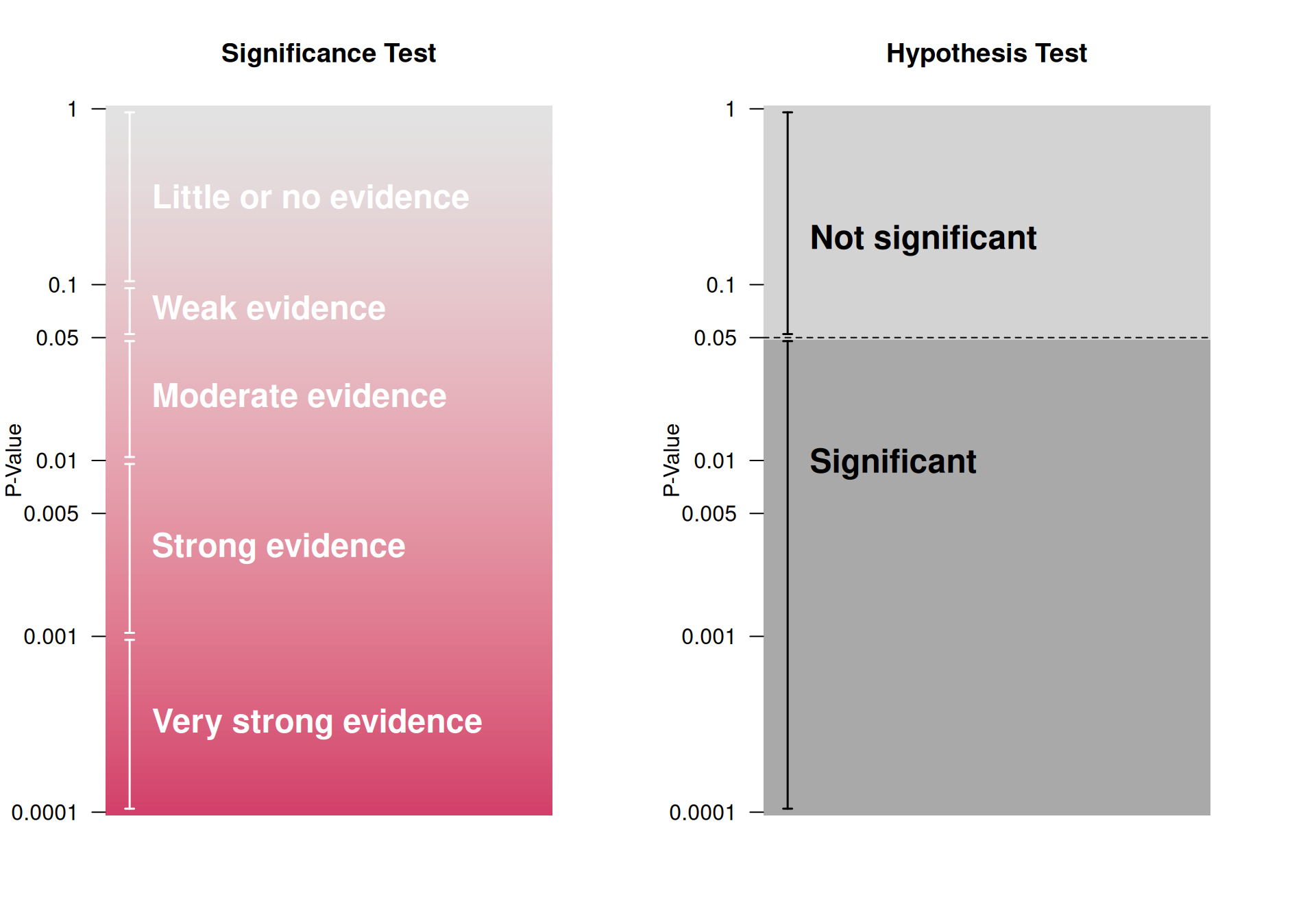
Figure 5.1: Significance vs Hypothesis Test, adapted from Bland (2015)
5.1.1 Computation of the \(P\)-value for a continuous outcome
The null hypothesis of no treatment effect can be expressed as:
\[\begin{eqnarray} H_0: \Delta = 0 \, , \end{eqnarray}\] with \(\Delta = \mu_1 - \mu_0\) denoting the difference in group means.
The test statistic
\[\begin{eqnarray*} z = \frac{\mbox{Estimate}}{\mbox{Standard error of the estimate}} \end{eqnarray*}\] quantifies how many standard errors the estimate of \(\Delta\) is away from the null. Most test statistics follow approximately a known reference distribution under the null hypothesis. Typical reference distributions include the standard normal distribution for large samples and the \(t\)-distribution for small samples, in which case the test statistic is usually denoted \(t\) rather than \(z\). The \(z\)-values can be used to compute the \(P\)-value: the larger the \(\left\lvert z\right\rvert\), the smaller the two-sided \(P\)-value.
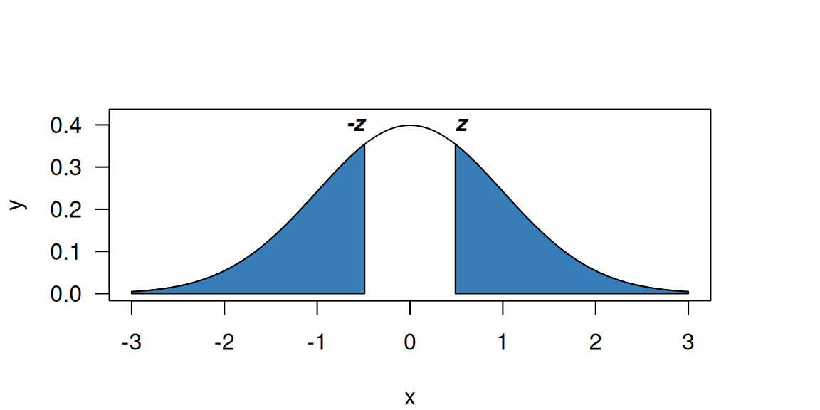
Figure 5.2: Two-sided p-value (blue region) for \(z=0.49\) and a standard normal reference distribution.
The \(P\)-value (for a \(z\)-value of \(z = 0.49\)) is graphically
illustrated in Figure 5.2.
The two-sided \(P\)-value is the area of the two blue regions
of the standard normal density, i.e. \(p = \Pr(\left\lvert Z\right\rvert > \left\lvert z\right\rvert) = 0.62\), where \(Z \sim \mathop{\mathrm{N}}(0, 1)\). In a two-sided test, only the
size of the effect matters, not its direction. In R, this can
be calculated with
## [1] 0.62Example 5.1 A study published in 1905 compared the effect of two soporific drugs on the increase in hours of sleep as compared to a control drug (Cushny and Peebles, 1905). The two drugs were given to ten individuals, so the data are paired and a two-sided paired \(t\)-test is used for the analysis. Data are shown in Figure 5.3.
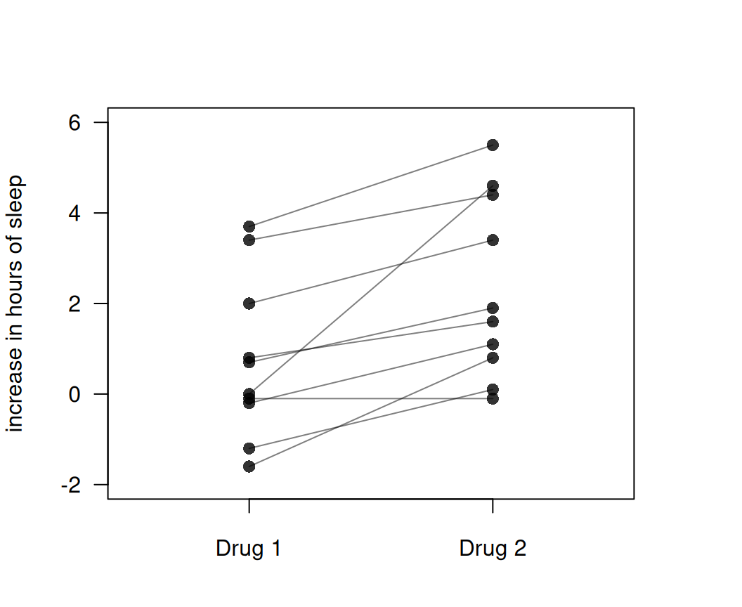
Figure 5.3: Increase in hours of sleep compared to control for two different drugs.
drug1 <- sleep$extra[sleep$group==1]
drug2 <- sleep$extra[sleep$group==2]
res <- t.test(drug1, drug2, data = sleep, paired = TRUE)
# extra: extra hours of sleep
# group: drug
print(res)
##
## Paired t-test
##
## data: drug1 and drug2
## t = -4.0621, df = 9, p-value = 0.002833
## alternative hypothesis: true mean difference is not equal to 0
## 95 percent confidence interval:
## -2.4598858 -0.7001142
## sample estimates:
## mean difference
## -1.58The two-sided \(P\)-value is \(p \approx 0.0028\), so there is strong evidence against the null hypothesis of no difference between the two drugs.
Example 5.2 In 1986, the data on 189 births were collected at Baystate Medical Center, Springfield, with the aim to identify risk factors associated with a low birthweight (Hosmer and Lemeshow, 1989). Let us assume that we are interested in knowing the impact of the smoking status of the mother on the baby weight at birth. Figure 5.4 shows the baby birthweight for smoking and non-smoking mothers.
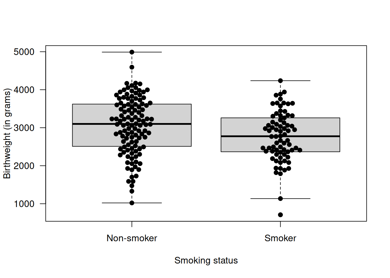
Figure 5.4: Birthweight of the baby as a function of the smoking status of the mother during the pregnancy.
##
##  Two Sample t-test
##
## data:  bwt by smoke
## t = 2.6529, df = 187, p-value = 0.008667
## alternative hypothesis: true difference in means between group 0 and group 1 is not equal to 0
## 95 percent confidence interval:
##   72.75612 494.79735
## sample estimates:
## mean in group 0 mean in group 1
##        3055.696        2771.919
A \(t\)-test can be conducted and the resulting \(P\)-value \(p = 0.0087\) indicates that there is evidence for a difference in mean birthweight between babies whose mother smoked and did not smoke during the pregnancy.
In two-sided tests, differences between treatment groups in either direction provide evidence against the null hypothesis. In contrast, only differences in a pre-specified direction provide evidence against the null in one-sided tests. If the difference goes in the expected direction, the one-sided \(P\)-value is half of the two-sided \(P\)-value, so \(\tilde p = p/2\). If not, \(\tilde p = 1 - p/2\). However, there is a risk of cheating by defining the test direction after having seen the data. For this reason, two-sided significance tests are the standard in clinical research.
Example 5.2 (continued) Now let us assume that the researchers expected the mean baby birthweight to be higher for non-smoking as compared to smoking mothers. In that case, one can calculate a one-sided \(P\)-value as follows
res.baby2 <- t.test(bwt ~ smoke, data = birthwt,
                    alternative = "greater", var.equal = TRUE)
print(res.baby2)
##
## Two Sample t-test
##
## data: bwt by smoke
## t = 2.6529, df = 187, p-value = 0.004333
## alternative hypothesis: true difference in means between group 0 and group 1 is greater than 0
## 95 percent confidence interval:
## 106.9528 Inf
## sample estimates:
## mean in group 0 mean in group 1
## 3055.696 2771.919The one-sided \(P\)-value \(\tilde p = 0.004\) is half the two-sided \(P\)-value as the difference in means goes in the expected direction.
res.baby3 <- t.test(bwt~ smoke, data = birthwt,
                    alternative = "less", var.equal = TRUE)
print(res.baby3)
##
## Two Sample t-test
##
## data: bwt by smoke
## t = 2.6529, df = 187, p-value = 0.9957
## alternative hypothesis: true difference in means between group 0 and group 1 is less than 0
## 95 percent confidence interval:
## -Inf 460.6007
## sample estimates:
## mean in group 0 mean in group 1
## 3055.696 2771.919In contrast, if researchers expect the mean baby birthweight to be higher for smoking as compared to non-smoking mothers, the one-sided \(P\)-value is \(\tilde p = 1 - p/2 \approx 1.00\).
5.1.2 Confidence intervals and \(P\)-values
Confidence intervals can be used to carry out a hypothesis test: If (and only if) the 95% CI does not contain the reference value, then the corresponding test is significant (two-sided p < 0.05). Furthermore, it is possible to transform a \(P\)-value to a confidence interval, provided that the effect estimate is known, the exact \(P\)-value is reported and is based on a normal test statistic (Altman and Bland, 2011a). Conversely, a confidence interval can be transformed to a \(P\)-value provided that the CI is of Wald-type (Altman and Bland, 2011b).
Example 5.2 (continued) The 95% confidence interval for the difference in mean baby birthweight between non-smoking and smoking mothers is \([72.76, 494.8]\). The approximate two-sided \(P\)-value can be retrieved using:
library(biostatUZH)
l <- 72.76
u <- 494.80
## estimate is in the middle of the confidence intervals
estimate <- (u + l)/2; print(estimate)
## [1] 283.78## standard error can be retrieved from width of confidence interval
se <- (u - l)/(2*1.96); print(se)## [1] 107.6633## z-statistic
z_val <- estimate/se
## two-sided p-value
p <- 2*pnorm(z_val, lower.tail=FALSE); print(p)## [1] 0.008393651The exact \(p\)-value based on the \(t\)-distribution is \(p = 0.0087\), so only slightly larger, see Example 5.2.
Confidence intervals convey very different information than \(P\)-values, see Figure 5.6 for illustration. Both quantities should be reported.
5.1.3 Error rates
Definition 5.2 Error rates
- The Type-I error rate \(\alpha\) is the probability of a significant finding if the null hypothesis \(H_0\) is true. The Type-I error rate is controlled at level \(\alpha\), if we reject \(H_0\) if and only if \(p \leq \alpha\).
- The Type-II error rate \(\beta\) is the probability of a non-significant finding if the alternative hypothesis \(H_1\) is true. The power of a study is \(1-\beta\). Power computations need a particular value for \(H_1\), e.g. \(H_1:`` \mbox{ true difference is 3.5 units}"\).
- Error rates are also useful for sample size calculations, see Section 5.2.
It is useful to compare hypothesis tests to diagnostic tests discussed in Chapter 1. If we consider a significant test result as a positive test and equate the null hypothesis of no effect with a non-diseased person then we see the following equivalences:
| Hypothesis test | Diagnostic test |
|---|---|
| Type-I error rate | \(1 - \text{Specificity}\) |
| Type-II error rate | \(1 - \text{Sensitivity}\) |
| Power | \(\text{Sensitivity}\) |
| False positive report probability | \(1 - \text{Positive predictive value}\) |
5.1.4 Misinterpretation of Type I Error
The \(P\)-value is not the only concept which suffers from misinterpretation; the Type-I error does too. Namely, \[ \alpha = \underbrace{\Pr(\mbox{significance} \,\vert\,H_0)}_{\tiny \mbox{Type I error rate}} \neq \underbrace{\Pr(H_0 \,\vert\,\mbox{significance})}_{\tiny \mbox{False positive report probability}}. \]
Although it is a mathematically trivial result, the misinterpretation of the Type I error rate \(\alpha\) as false positive report probability is very common. For example, Giesecke (2002) claims that a 5% significance level “means that out of 20 studies reporting significant associations, one will just be a chance finding”. This statement is wrong, and confuses the Type I error rate with the false positive report probability.
The false positive report probability can be calculated as
\[\begin{eqnarray} \tag{5.1} \mbox{FPRP} = \frac{\Pr(H_0) \cdot \alpha}{\Pr(H_0) \cdot \alpha + \Pr(H_1) \cdot (1 - \beta)} \, . \end{eqnarray}\]
Suppose that a number of trials are performed and consider two scenarios: 10% of the trials are truly effective in scenario 1 (\(\Pr(H_1) = 0.1\)), and 70% in scenario 2 (\(\Pr(H_1) = 0.7\)). The Type-I error rate and the power are fixed to \(\alpha = 0.05\) and \(1 - \beta = 0.8\), respectively, in both scenarios. Using Equation (5.1), the false positive report probability is \(36\)% in the first scenario and \(3\)% in the second. While the Type-I error rate is fixed and the same in both scenarios, the false positive report probability is very different as it depends on the power and the probability of \(H_1\).
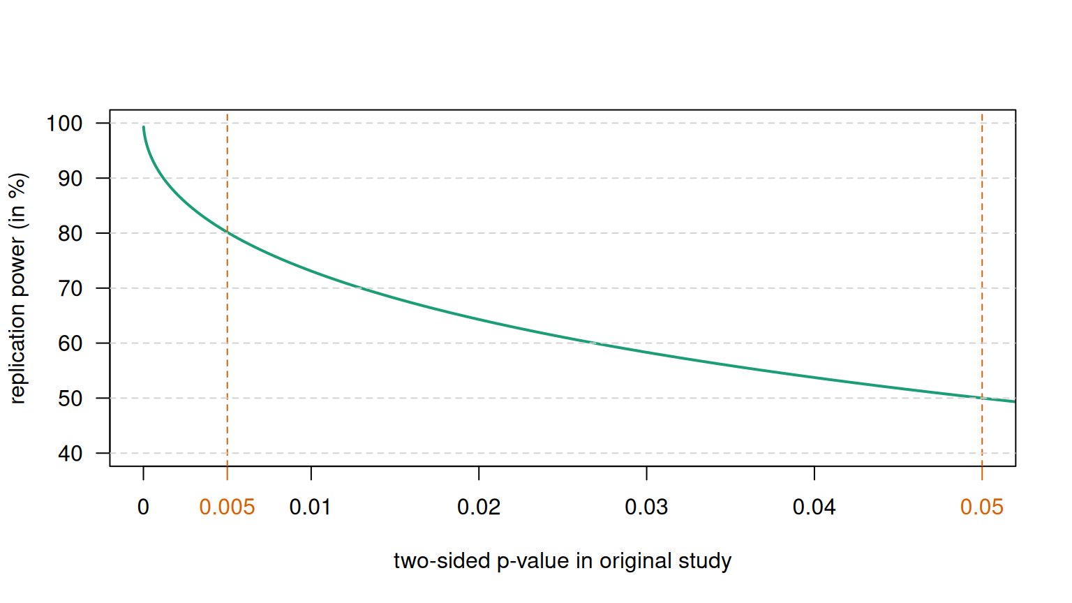
Figure 5.5: Replication power as a function of the \(P\)-value.
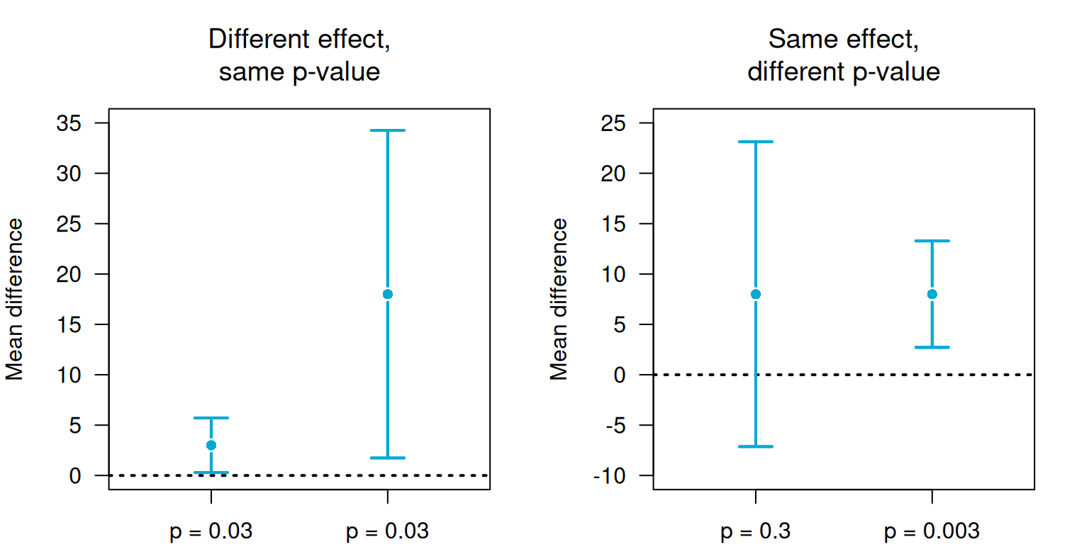
Figure 5.6: P-values and confidence intervals convey different information.
5.2 Sample size calculations
Having a fixed target for recruitment implies that you have a known objective stopping rule. Appropriate sample size calculations ensure that enough patients are recruited to collect statistical evidence for a treatment effect and that the number of patient treated with inferior treatment is not unnecessarily large.
Sample size calculations require the specification of the primary outcome variable (“primary endpoint”). A (minimal) clinically relevant treatment effect \(\Delta\) (“clinically relevant difference”) for the primary outcome also needs to be specified in advance.
Definition 5.3 The minimal clinically relevant difference is the smallest difference of the primary outcome variable that clinicians and patients would care about.
Example 5.3 Doyle et al (2024) conducted an RCT to test whether an intensive food-as-medicine program for patients with diabetes improves glycemic control. The primary outcome was hemoglobin A\(_{\small{1c}}\) level at six months, and the minimal clinically relevant difference was \(\Delta = -0.5\)-percentage points in hemoglobin A\(_{\small{1c}}\) levels. Secondary outcomes included other biometric measures and healthcare use, among others.
5.2.1 Continuous outcomes
Suppose two independent equally sized groups are to be compared. In order to derive the sample size formula, four quantities are required:
- Clinically relevant difference \(\Delta = \mu_1 - \mu_0\)
- Common standard deviation \(\sigma\) (measurement error)
- Type-I error rate \(\alpha \rightarrow u = z_{1 - \alpha/2}\), where \(z_x =\)
qnorm(x) - Power \(1 - \beta \rightarrow v = z_{1 - \beta}\).
The required sample size \(n\) per group is then
\[\begin{eqnarray} \tag{5.2} n = \frac{ 2 \sigma^2 (u + v)^2}{ \Delta^2} = \frac{ 2 (u + v)^2}{ \left(\Delta/\sigma\right)^2} \, , \end{eqnarray}\]
where Cohen’s \(d\) \(=\Delta/\sigma\) is the relative difference
in terms of standard deviations \(\sigma\). Formula (5.2) is implemented in the function biostatUZH::power.z.test().
The classification of Cohen’s \(d\) and the corresponding AUC can be found in Table 5.1 and are illustrated in Figure 5.7.
| Cohen’s effect size \(d\) | AUC | Interpretation |
|---|---|---|
| 0.0 | 0.50 | Null |
| 0.2 | 0.56 | Small |
| 0.5 | 0.64 | Medium |
| 0.8 | 0.71 | Large |
| 1.3 | 0.82 | Very large |
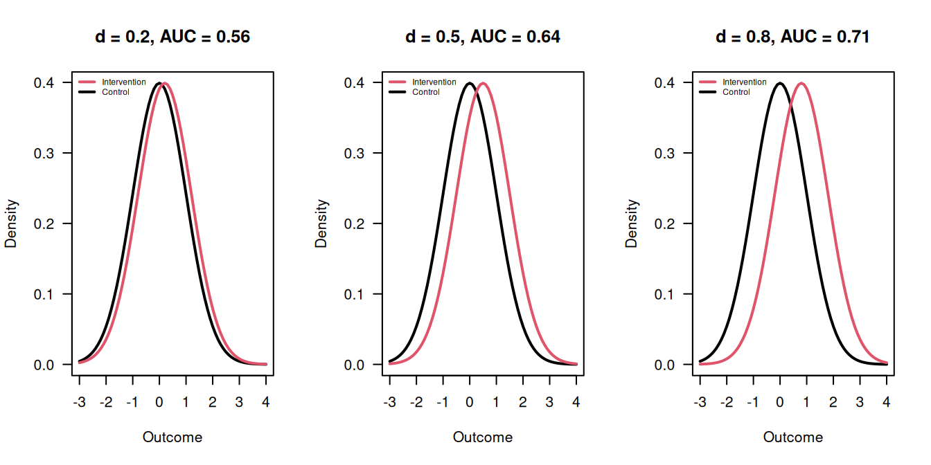
Figure 5.7: Outcomes in the Intervention and Control groups for \(d = 0.2\), \(d = 0.5\) and \(d = 0.8\).
Suppose that \(d = 1\), so the clinically relevant difference \(\Delta\) equals the standard deviation \(\sigma\) of the measurements. Table 5.2 gives for this case the required sample size \(n=2(u+v)^2\) in each group. The numbers have to be adjusted for different values of \(d\). For example, if \(d = 1/2\) then the numbers have to be multiplied with 4.
| \(\alpha\) | \(\beta\) | \(u\) | \(v\) | \((u + v)^2\) | Group sample size \(n\) |
|---|---|---|---|---|---|
| 5% | 20% | 1.96 | 0.84 | 7.8 | 15.7 |
| 5% | 10% | 1.96 | 1.28 | 10.5 | 21.0 |
| 1% | 20% | 2.58 | 0.84 | 11.7 | 23.4 |
| 1% | 10% | 2.58 | 1.28 | 14.9 | 29.8 |
Example 5.4 A randomized controlled trial is conducted to assess the clinical and cost effectiveness of conservative management compared with laparoscopic cholecystectomy for the prevention of symptoms and complications in adults with uncomplicated symptomatic gallstone disease (Ahmed et al, 2023). A clinically relevant effect of \(0.33\) standard deviations was selected. A Type-I error rate of \(\alpha = 0.05\) and a power of \(1 - \beta = 0.90\) were agreed on.
##
##      Two-sample z test power calculation
##
##               n = 192.9738
##           delta = 0.33
##              sd = 1
##       sig.level = 0.05
##           power = 0.9
##     alternative = two.sided
##
## NOTE: n is number in *each* group
\(n = 193\) patients are needed in each group.
Exact calculations based on the t-test give a slightly larger value for \(n\), which corresponds to the value given in Ahmed et al (2023):
## [1] 193.9392The exact statement in the paper reads: “A sample size of 194 in each group was needed to detect a mean difference in area under the curve of 0.33 standard deviations derived from the SF-36 bodily pain domain with 90% power and a 5% (two-sided \(\alpha\)) significance level.”
Minimum detectable difference
Definition 5.4 The minimum detectable difference (MDD) is the smallest difference that will lead to a significant result:
\[ \mbox{MDD} = \sigma \sqrt{2/n} \cdot u. \]
The MDD and the clinically relevant difference \(\Delta\) are different concepts which should not be mixed up. The MDD relates to the statistical significance, hence depends on power (via the sample size), while \(\Delta\) relates to the clinical relevance and does not depend on the power. Suppose that the sample size \(n\) is calculated to detect \(\Delta\) with a certain power using Equation (5.2). Figure 5.8 compares the minimum detectable difference MDD as a function of that power to the minimal clinically relevant difference \(\Delta\). If the power \(>50\%\), then MDD \(<\Delta\).
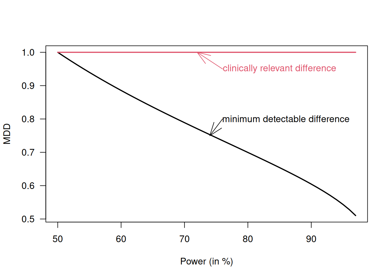
Figure 5.8: Minimum detectable difference is smaller than the (minimal) clinically relevant difference \(\Delta\) if the trial is powered for \(>50\%\)
5.2.2 Binary outcomes
In order to calculate the sample size for a binary outcome,
the outcome probabilities \(\pi_1\) and \(\pi_0\) in the two groups
are needed. The clinically relevant difference
\(\Delta = \pi_1 - \pi_0\) is then implicit. No standard deviation
is required.
The
required sample size per group can be calculated using
biostatUZH::power.prop.test().
An alternative approach based on the variance stabilizing (angular) transformation \(h(\pi) = \arcsin(\sqrt{\pi})\) is described in Matthews (2006) (Sec. 3.4) where the sample size per group is
\[ n = \frac{(u+v)^2}{2\{h(\pi_1) - h(\pi_0)\}^2}. \]
This corresponds to the traditional formula for continuous outcomes with clinically relevant difference \(\Delta = h(\pi_1) - h(\pi_0)\) and standard deviation \(\sigma = 1/2\).
Example 5.5 An RCT was conducted to investigate the effectiveness of oral antimicrobial prophylaxis on surgical site infection after elective colorectal surgery (Futier et al, 2022). The primary outcome was the proportion of patients with surgical site infection within 30 days after surgery, and a difference in proportion of \(\Delta = 15\% - 9\% = 6\%\) was considered clinically relevant. A power of 80% and Type-I error rate of 5% were agreed on.
The required sample size can be calculated using R:
##
##      Two-sample comparison of proportions power calculation
##
##               n = 459.2869
##              p1 = 0.15
##              p2 = 0.09
##       sig.level = 0.05
##           power = 0.8
##     alternative = two.sided
##
## NOTE: n is number in *each* group
The statement in the paper is: “Assuming a 15% rate of surgical site infections with placebo, we estimated that enrolling 920 patients would provide 80% power to detect a 40% relative between group difference in the incidence of the primary outcome (i.e., 15% in the placebo group and 9% in the oral ornidazole group), with a 5% two-sided Type I error.”
The alternative approach based on the variance-stabilizing transformation gives a somewhat smaller sample size:
##
##      Two-sample z test power calculation
##
##               n = 453.679
##           delta = 0.09300676
##              sd = 0.5
##       sig.level = 0.05
##           power = 0.8
##     alternative = two.sided
##
## NOTE: n is number in *each* group
5.2.3 Adjusting for loss to follow-up
In practice, the calculated sample size \(n\) should be increased to allow for possible non-response or loss to follow-up. If a drop-out rate of \(x\) % can be anticipated, then we obtain the adjusted sample size \[ n^\star = \underbrace{\frac{100}{100-x}}_{\tiny \mbox{adjustment factor}} \cdot \,\, n \] For example, to incorporate a drop-out rate of 20%, we need to use an adjustment factor of \(100/80 = 1.25\).
In the study presented in Example 5.4, a drop-out rate of 10% was expected, so 430 patients were required. In Example 5.5, the sample size was inflated to 960 patients to account for a 5% loss to follow-up.
5.2.4 Study designs with unequal group sizes
In the case of equally sized groups with \(n\) patients each, the standard error of the estimate \(\hat \Delta\) is
\[\begin{equation} \tag{5.3} \mbox{se}(\hat \Delta) = {\sigma \sqrt{2/n}} \end{equation}\]
In the case of different sample sizes \(n_0\) and \(n_1\) with group size ratio \(c = n_1/n_0\), the term \({2/n}\) in (5.3) has to be replaced by \({1/n_0 + 1/n_1} = (1+c)/n_1\) and so
\[\begin{eqnarray*} n_1 &=& n \cdot (1+c)/ 2 \\ n_0 & = & n_1/c \end{eqnarray*}\]
where \(n\) is the required sample size for equal-sized groups. The total sample size \(n_0+n_1\) increases with increasing ratio \(c\), as illustrated in Figure 5.9. This indicates that the greater the imbalance, the larger the total sample size needs to be.
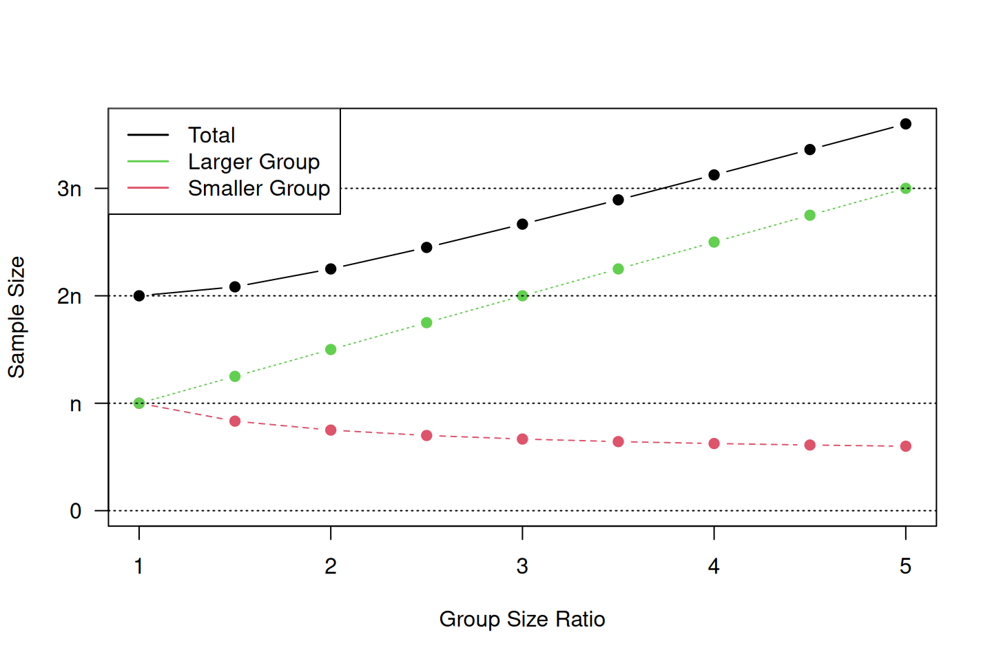
Figure 5.9: Required sample size depending on the group size ratio for study designs with unequal group sizes.
5.2.5 Sample size based on precision
It has been argued in Bland (2009) that sample size calculations should be based on precision, i.e. the width of the confidence interval of the treatment effect.
Difference between two means
Specify the width \(w \approx 4 \cdot \mbox{se}(\hat \Delta)\) of the 95% confidence interval for the mean difference \(\Delta\). Both groups are assumed to have sample size \(n\).
With \(\mbox{se}(\hat \Delta) = \sigma \sqrt{2/n}\), we obtain for the sample size in each group: \[ n = 2 \, \frac{\sigma^2}{\mbox{se}(\hat \Delta)^2} = 32 \, \frac{\sigma^2}{w^2} \, . \] For example, if the width \(w\) is required to be half as large as \(\sigma\), the sample size per group is \(n=128\).
Difference between two proportions
If \(\Delta=\pi_1-\pi_o\) is the difference between two proportions \(\pi_1\) and \(\pi_0\) with unit variance \[ \sigma^2 = \{\pi_1 (1-\pi_1) + \pi_0 (1-\pi_0)\}/2, \] the required sample size in each group is \[ n = \frac{\sigma^2}{\mbox{se}(\hat \Delta)^2}= 16 \, \frac{\sigma^2}{w^2} \, , \] where \(w = 4 \mbox{se}(\hat \Delta)\) is the width of the 95% confidence interval for \(\Delta\). For example, if \(\pi_1=0.2\), \(\pi_0=0.05\) and \(w=0.1\), then \(n=332\).
5.2.6 Sample size re-estimation
There are various assumptions that can impact sample size calculation. For example, higher-than-expected variance may reduce the power to detect treatment effects. We can use sample size re-estimation at interim analysis, for example re-estimating the standard deviation \(\sigma\) in internal pilot, or potentially increase sample size to maintain power level. We can also adjust sample size for “blinded” vs. “unblinded” designs (with respect to treatment assignment). Other parameters can also be re-estimated, for example the baseline event rate parameter for binary outcomes. For more discussions, see Chuang-Stein et al (2006) and Proschan (2009).
5.3 Additional references
Significance tests and and sample size determination are discussed in Bland (2015) (Chapters 9 and 18). Specifically for RCTs, Matthews (2006) (Chapter 3) discusses the question of “how many patients do I need”. Studies where the methods from this chapter are used in practice are for example Freedman et al (2011), Heal et al (2009) and Wen et al (2012).