Chapter 15 Meta-analysis
Results from a single study are not sufficient to detect or exclude a relevant effect of a new therapy. Meta-analysis describes statistical techniques to summarize the effect estimates obtained from several independent studies on the same research question (Schmid et al, 2021). The studies included in a meta-analysis are usually the result of a systematic review (Egger et al, 2022). There are also narrative systematic reviews where a subsequent meta-analysis is not possible.
15.1 Systematic review
A systematic review aims to identify relevant studies from a literature review. This is usually done with a literature search with pre-defined search terms in a database such as MEDLINE. Results from unpublished studies may also be included, if they are available from platforms such as clinicaltrials.gov. The goal of a subsequent meta-analysis is to summarize the results from a number of clinical studies on the same research question. A systematic review with subsequent meta-analysis proceeds as follows:
- Systematically review the available evidence.
- Provide quantitative summaries of the results from each study.
- Combine these results across studies, if appropriate (meta-analysis).
- Provide summary effect estimate.
This is the basis of evidence-based medicine (EBM). The studies included in a systematic review should be sufficiently homogeneous regarding in- and exclusion criteria and should use the same effect measure. A typical effect measure for continuous outcomes is the (standardized) difference in means \(\theta\) between treatment groups. For binary/time to event outcomes, relative treatment effects are preferred, such as relative risk \(\mbox{RR}\), odds ratio \(\mbox{OR}\) and hazard ratio \(\mbox{HR}\). These are usually considered on a log-scale, so the relevant effect estimate is \(\theta=\log(\mbox{RR})\), \(\theta=\log(\mbox{OR})\), \(\theta=\log(\mbox{HR})\).
Example 15.1 Consider nine RCTs studying the incidence of preeclampsia in patients treated with diuretic versus a control treatment. The reported effect measure is an odds ratio (diuretic vs. control), see Table 15.1.
| Study | Diuretic | Control | OR |
|---|---|---|---|
| Weseley | 11% (14/131) | 10% (14/136) | 1.04 |
| Flowers | 5% (21/385) | 13% (17/134) | 0.40 |
| Menzies | 25% (14/57) | 50% (24/48) | 0.33 |
| Fallis | 16% (6/38) | 45% (18/40) | 0.23 |
| Cuadros | 1% (12/1011) | 5% (35/760) | 0.25 |
| Landesman | 10% (138/1370) | 13% (175/1336) | 0.74 |
| Krans | 3% (15/506) | 4% (20/524) | 0.77 |
| Tervila | 6% (6/108) | 2% (2/103) | 2.97 |
| Campbell | 42% (65/153) | 39% (40/102) | 1.14 |
Figure 15.1 shows a graphical summary of the log odds ratios with 95% CIs. This kind of graphical summary is called a forest plot.
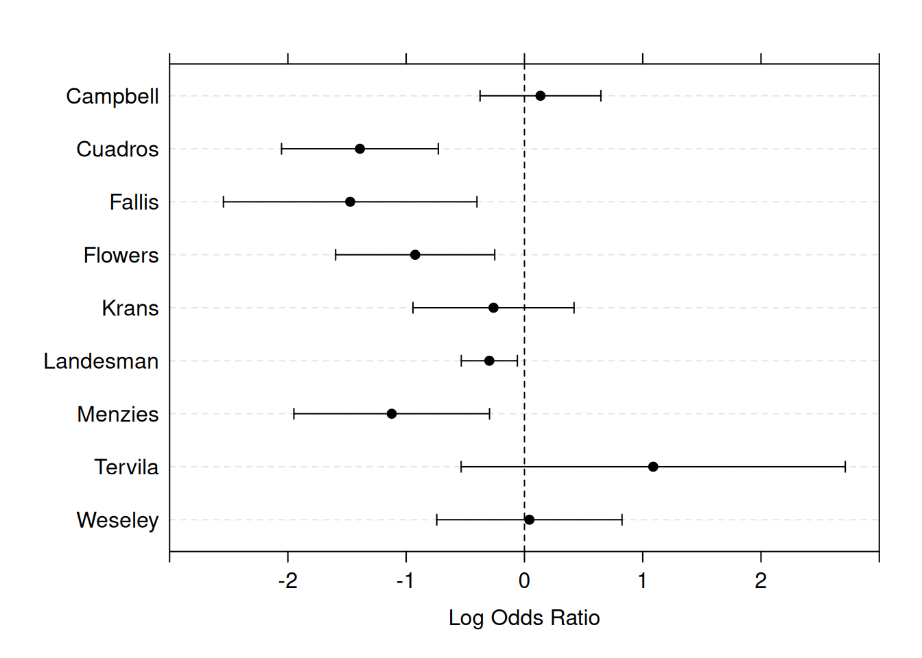
Figure 15.1: Forest plot for the estimated effects with 95% confidence intervals in the nine studies from Example 15.1.
15.2 Meta-analysis
We set the following notation for a meta-analysis of \(i=1,\ldots, n\) trials:
- \(\theta_i\), \(\hat \theta_i\) are the true and estimated study-specific treatment effect,
- \(s_i = \mathop{\mathrm{se}}(\hat \theta_i)\) is the standard error of \(\hat \theta_i\),
- \(v_i = s_i^2\) is the variance of \(\hat \theta_i\).
There are two different types of analyses: fixed and random effects model.
15.2.1 Fixed effect model
A fixed effect model is based on the homogeneity assumption: \(\theta_i = \theta\) for all \(i\). The estimate \(\hat \theta\) of the overall treatment effect \(\theta\) is then a weighted average of study-specific estimates \(\hat \theta_i\) with inverse variance weights \(w_i=1/v_i\):
\[\begin{equation*} \hat \theta = \frac{\sum w_i \hat \theta_i}{\sum w_i} \mbox{ with } \mathop{\mathrm{se}}(\hat \theta) = 1/\sqrt{\sum w_i}. \end{equation*}\]
The overall effect is usually displayed in the forest plot, as in
Figure 15.2 for the preeclampsia
Example 15.1. This figure is generated with the following
R code:
library(meta)
meta1 <- metabin(event.e = treatedPre, n.e = treatedTot,
                 event.c = controlPre, n.c = controlTot,
                 sm = "OR" , method = "Inverse", studlab = study)
forest(meta1, comb.fixed = TRUE, comb.random = TRUE) 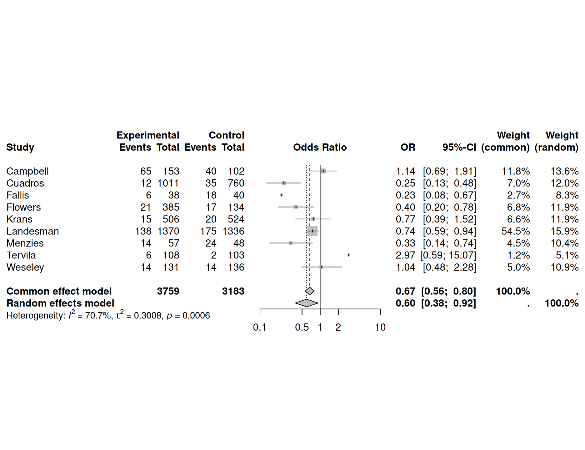
Figure 15.2: Results with forest plot from package meta for a fixed effect analysis in Example 15.1
Cochran’s test for heterogeneity
Under the homogeneity assumption, we have
\[\begin{equation*} Q = \sum w_i (\hat \theta_i - \hat \theta)^2 \mathrel{\overset{\text{a}}{\thicksim}}\chi^2_{n-1} \end{equation*}\]
This can be used to calculate the \(P\)-value of Cochran’s test for heterogeneity.
Example 15.1 (continued) For the preeclampsia data, this test yields \(Q = 27.3\) at \(n-1=8\) degrees of freedom (\(p=0.00064\)). There is strong evidence for heterogeneity between studies, so a fixed effect model is questionable.
15.2.2 Random effects model
A random effects model assumes that the \(\theta_i\)’s come from a normal distribution with mean \(\theta^*\) and heterogeneity variance \(\tau^2\):
\[\begin{equation*} \hat \theta_i \,\vert\,\theta_i \sim \mathop{\mathrm{N}}(\theta_i, v_i) \quad \mbox{ and } \quad \theta_i \sim \mathop{\mathrm{N}}(\theta^*, \tau^2), \end{equation*}\]
so marginally
\[\begin{equation*} \hat \theta_i \sim \mathop{\mathrm{N}}(\theta^*, v_i + \tau^2). \end{equation*}\]
The overall effect estimate \(\hat \theta^*\) and its standard error are now:
\[\begin{equation*} \hat \theta^* = \frac{\sum w_i^* \hat \theta_i}{\sum w_i^*}, \quad \mathop{\mathrm{se}}(\hat \theta^*) = {1}/{\sqrt{\sum w_i^*}}, \end{equation*}\]
with weights \(w_i^* = {1}/{(v_i + \tau^2)}\). Compared to the fixed effect model, the CIs for the overall effect will become wider and large studies will obtain less weight.
Estimate of heterogeneity variance and Higgins’ \(I^2\)
The moment estimator of the heterogeneity variance compares the \(Q\)-statistic to its expectation \(n-1\) under homogeneity. Truncation at zero and appropriate scaling gives
\[\begin{equation*} \hat \tau^2 = \left\{Q-(n-1)\right\}_{+} / \left\{\textstyle\sum w_i - \textstyle\sum w_i^2/\textstyle\sum w_i\right\}. \end{equation*}\]
The standard DerSimonian-Laird approach plugs \(\hat \tau^2\) in \(w_i^* = {1}/{(v_i + \tau^2)}\), the alternative Hartung-Knapp adjustment accounts for the uncertainty of \(\hat \tau^2\).
Easier to interpret is Higgins’ \(I^2\), the percentage of variance that is attributable to study heterogeneity. The value of \(I^2\) will somewhat depend on the method used to estimate \(\tau^2\), although in practice this aspect can be neglected.
Figure 15.2 also shows the results of a random effects analysis, together with the estimated Higgins’ \(I^2\) and heterogeneity variance \(\tau^2\).
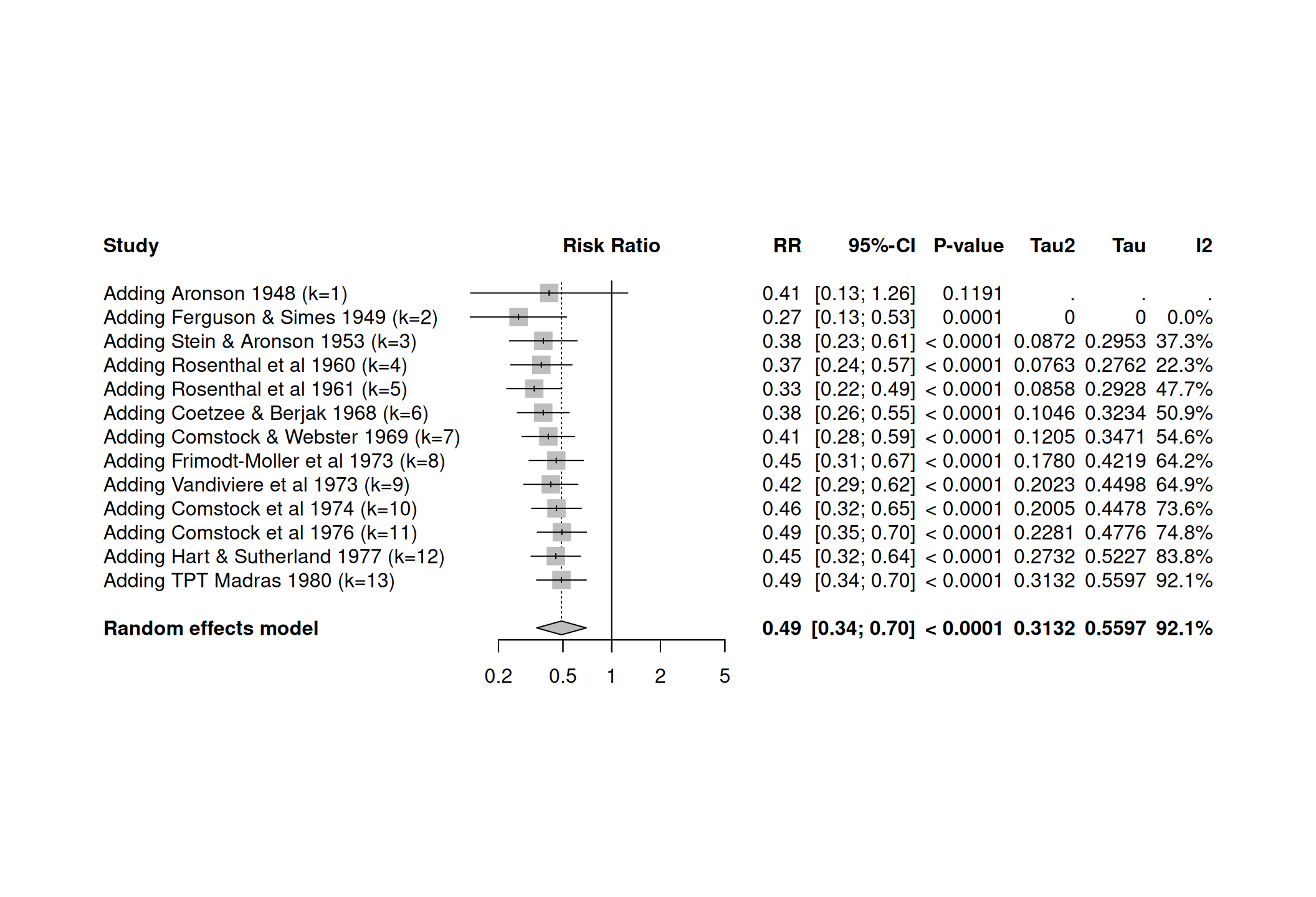
15.2.3 Cumulative meta-analysis
A cumulative meta-analysis plot shows how evidence has accumulated over time. The \(i\)-th line in a cumulative meta-analysis plot is the summary produced by a meta-analysis of the first \(i\) trials.
Example 15.2 The dataset dat.bcgfrom the Rpackage metadat
gives the results from 13 studies examining the effectiveness
of the Bacillus Calmette-Guerin (BCG) vaccine
against tuberculosis.
The meta-analysis can be performed with the function
meta::metabin():
meta1 <- metabin(event.e = tpos, n.e = tpos + tneg,
event.c = cpos, n.c = cpos + cneg, data=dat.bcg, sm = "RR",
method = "Inverse", studlab = paste(author, year))
### Forest plot
forest(meta1)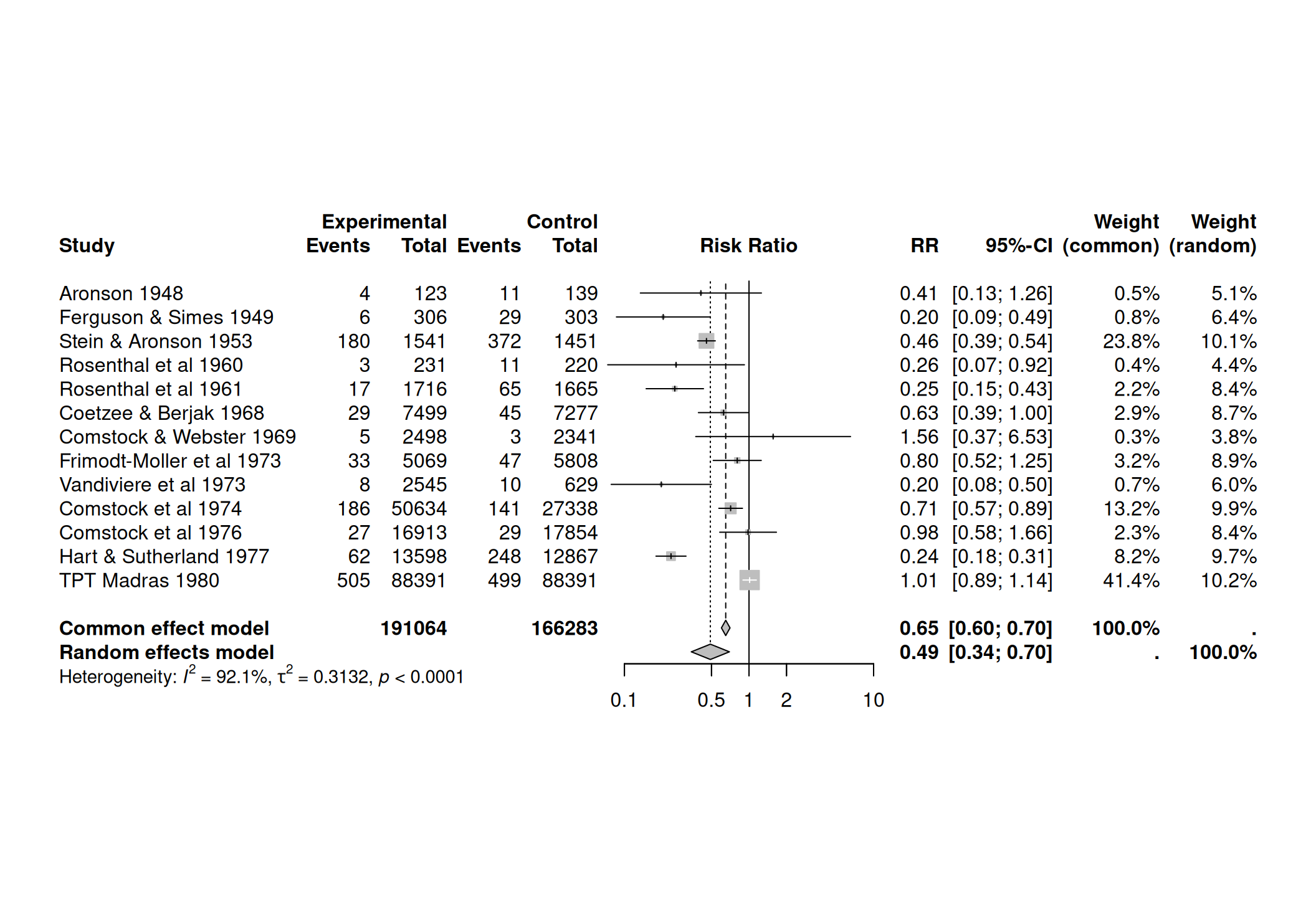 The cumulative meta-analysis can be performed with the function
meta::metacum():
15.2.4 Meta-regression
A meta-regression tries to explain heterogeneity with study-specific covariates. The visualization can be done with bubble plots.
Example 15.2 (continued) In the dat.bcg dataset, the covariable ablat gives the absolute
latitude of the study location (in degrees), and can possibly be
a relevant moderator of the effectiveness of the vaccine.
The meta-regression can be performed with the function
meta::metareg():
##
## Mixed-Effects Model (k = 13; tau^2 estimator: REML)
##
## tau^2 (estimated amount of residual heterogeneity):     0.0764 (SE = 0.0591)
## tau (square root of estimated tau^2 value):             0.2763
## I^2 (residual heterogeneity / unaccounted variability): 68.39%
## H^2 (unaccounted variability / sampling variability):   3.16
## R^2 (amount of heterogeneity accounted for):            75.62%
##
## Test for Residual Heterogeneity:
## QE(df = 11) = 30.7331, p-val = 0.0012
##
## Test of Moderators (coefficient 2):
## QM(df = 1) = 16.3571, p-val < .0001
##
## Model Results:
##
##          estimate      se     zval    pval    ci.lb
## intrcpt    0.2515  0.2491   1.0095  0.3127  -0.2368
## ablat     -0.0291  0.0072  -4.0444  <.0001  -0.0432
##            ci.ub
## intrcpt   0.7397
## ablat    -0.0150  ***
##
## ---
## Signif. codes:  0 '***' 0.001 '**' 0.01 '*' 0.05 '.' 0.1 ' ' 1
The function meta::bubble() produces the bubble plot.
par(las=1)
bubble(mr1, lwd = 2, col.line = "blue", studlab=TRUE, xlim=c(-5, 60),
       cex.studlab=0.7, ylim=c(0.15, 1.8))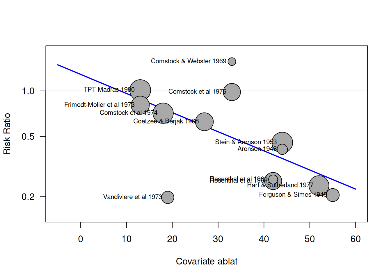
15.3 Reporting bias
Reporting bias occurs when the publication of research results depends on their nature and direction. Sources of reporting bias include publication bias (where studies with negative or null findings may not be published due to decisions by researchers, referees, editors, or journals), language bias, citation bias, time lag bias, and outcome reporting bias (where outcomes are selectively reported, often due to changes in the research plan). These biases can lead to false conclusions and potentially harm patients.
15.3.1 Funnel plot
A funnel plot is a scatter plot of a measure of study size, usually the (reversed) standard error, against the estimated treatment effects from individual studies. The funnel plot for the preeclampsia data is shown in Figure 15.3.
The smaller the study size, the wider the spread of the treatment effects and vice versa. If there is no bias, the point cloud has the form of a funnel (symmetrical). In contrast, it is asymmetrical
if there is bias. However, it is an explorative tool and there is no quantitative information on the amount or the source of the bias.
Funnel plots and tools for meta-analysis in R are provided by the packages meta and rmeta.

Figure 15.3: Funnel plot for preeclampsia data from Example 15.1
Example 15.3 Hackshaw (1998) conducted a meta-analysis of 37 studies of the effect of environmental tobacco smoke on the risk of lung cancer in lifetime non-smokers. Spouses of smokers and non-smokers have been compared in terms of log relative risk. Are the results shown in a funnel plot in Figure 15.4 affected by publication bias?
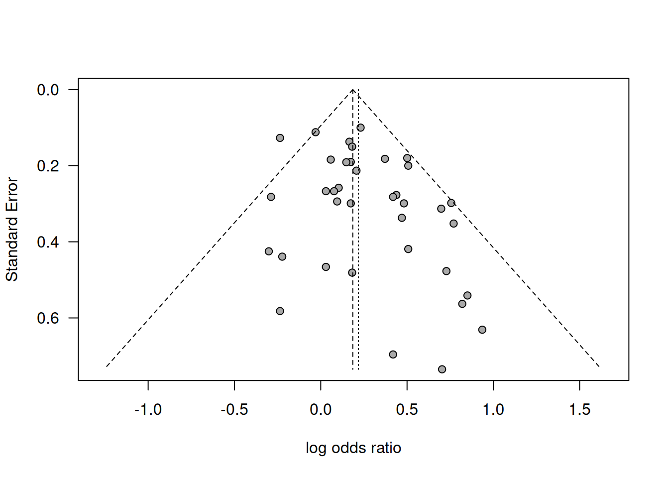
Figure 15.4: Funnel plot of results in the meta-analysis about risk of lung cancer from passive smoking by Hackshaw (1998).
Smaller studies tend to show greater effects, so there is some asymmetry. However, only visual inspection is not enough to decide if it is real bias or due to chance.
15.3.2 The trim-and-fill method
The trim-and-fill method is based on the key assumptions that publication bias is the reason of funnel plot asymmetry and that the studies with negative findings are suppressed. The idea of this method is to:
- Trim-off the “asymmetric” side of a funnel plot, after estimating the number of studies in this group.
- Use the symmetric remainder to estimate the “true center”.
- Impute trimmed studies and their missing “counterparts” around the center.
- Estimate \(\theta\) and its variance based on the “filled” funnel plot.
Example 15.4 Figure 15.5 illustrates the trim-and-fill method for 11 studies of the effect of using gangliosides in reducing case fatality and disability in acute ischemic stroke.
Figure 15.5: Trim-and-fill method in Example 15.4. The black circles represent the 11 observed studies whereas the red studies on the left are imputed, based on symmetrically mirroring the trimmed studies on the right.
Trim-and-fill with R:
library(meta) # load the library
gs <- as.matrix(read.table("data/ganglioside.txt", header = TRUE))
tf_gs <- trimfill(x = gs[,1], seTE = gs[,2],
ma.fixed = FALSE, type = "L", silent = TRUE)## Number of studies: k = 16 (with 5 added studies)
##
## 95%-CI z p-value
## Random effects model 0.0147 [-0.2037; 0.2332] 0.13 0.8948
##
## Quantifying heterogeneity (with 95%-CIs):
## tau^2 < 0.0001 [0.0000; 0.8626]; tau = 0.0022 [0.0000; 0.9288]
## I^2 = 0.0% [0.0%; 52.3%]; H = 1.00 [1.00; 1.45]
##
## Test of heterogeneity:
## Q d.f. p-value
## 14.88 15 0.4604
##
## Details of meta-analysis methods:
## - Inverse variance method
## - Restricted maximum-likelihood estimator for tau^2
## - Q-Profile method for confidence interval of tau^2 and tau
## - Calculation of I^2 based on Q
## - Trim-and-fill method to adjust for funnel plot asymmetry (L-estimator)Example 15.3 (continued) Data from the passive smoking example is illustrated in Figure 15.6. Results from the trim-and-fill method are shown in Figure 15.7. The summary effect with (in red) and without (in black) the results from the imputed studies is shown at the bottom.
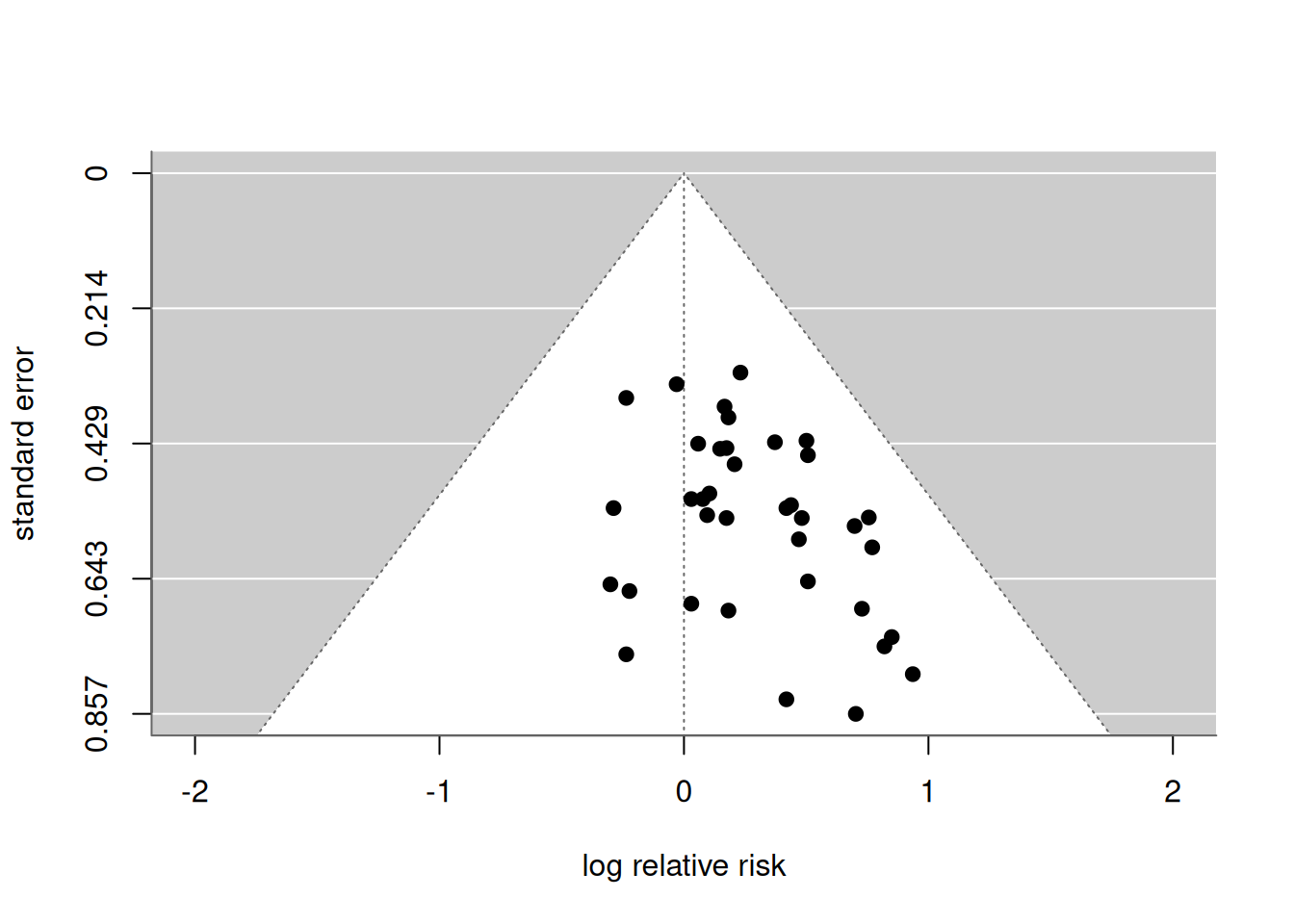
Figure 15.6: Funnel plot in the passive smoking Example 15.3.
| Model | Number of studies | OR | 95% CI |
|---|---|---|---|
| Observed | 37 | 1.24 | (1.13, 1.37) |
| Filled | 44 | 1.19 | (1.08, 1.31) |
Figure 15.7: Trim-and-fill method in the passive smoking Example 15.3.
15.3.3 Tests for funnel plot asymmetry
If visual inspection of a funnel plot is not enough, statistical tests can be performed. Popular methods are Begg’s rank correlation method or Egger’s test (weighted regression).
Begg’s rank correlation test
Begg’s rank correlation test computes standardized treatment estimates
\[\begin{equation*} \theta_i^*=\frac{\theta_i-\hat{\theta}}{\sqrt{v_i^*}}, \end{equation*}\]
where \(\hat{\theta}\) is the fixed-effect estimate of the summary effect and \(v_i^*=v_i - 1/(\sum v_j^{-1})\) is the variance of \(\theta_i-\hat{\theta}\). Then, it tests the null hypothesis that Kendall’s rank correlation (Kendqll’s \(\tau\)) between \(\theta_i^*\) and \(v_i^*\) is zero. This test may have low power if the number of studies is small.
A rank correlation test can be performed using R as shown below for Example 15.3.
##     lnRR selnRR
## 1  0.231  0.100
## 2 -0.030  0.112
## 3 -0.236  0.127
## 4  0.166  0.137
## 5  0.182  0.150
## 6 0.501 0.180## Rank correlation test of funnel plot asymmetry
##
## Test result: z = 1.27, p-value = 0.2044
## Bias estimate: 97.0000 (SE = 76.4395)
##
## Reference: Begg & Mazumdar (1993), BiometricsEgger’s weighted regression
The idea is to perform weighted regression of \(\hat \theta_i\) on \(s_i\),
\[\begin{equation*} \hat \theta_i= a + b \cdot s_i + \mbox{error}, \end{equation*}\]
with weights \(w_i = 1/s_i^2\). The slope \(b\) is a measure of bias.
Example 15.3 (continued) Egger’s weighted regression can be performed in R as shown below for the passive smoking example:
| Coefficient | 95%-confidence interval | \(p\)-value | |
|---|---|---|---|
| Intercept | 0.009 | from -0.16 to 0.18 | 0.92 |
| s | 0.89 | from 0.13 to 1.66 | 0.024 |
Figure 15.8 shows a visualization of Egger’s weighted regression in the passive smoking example.
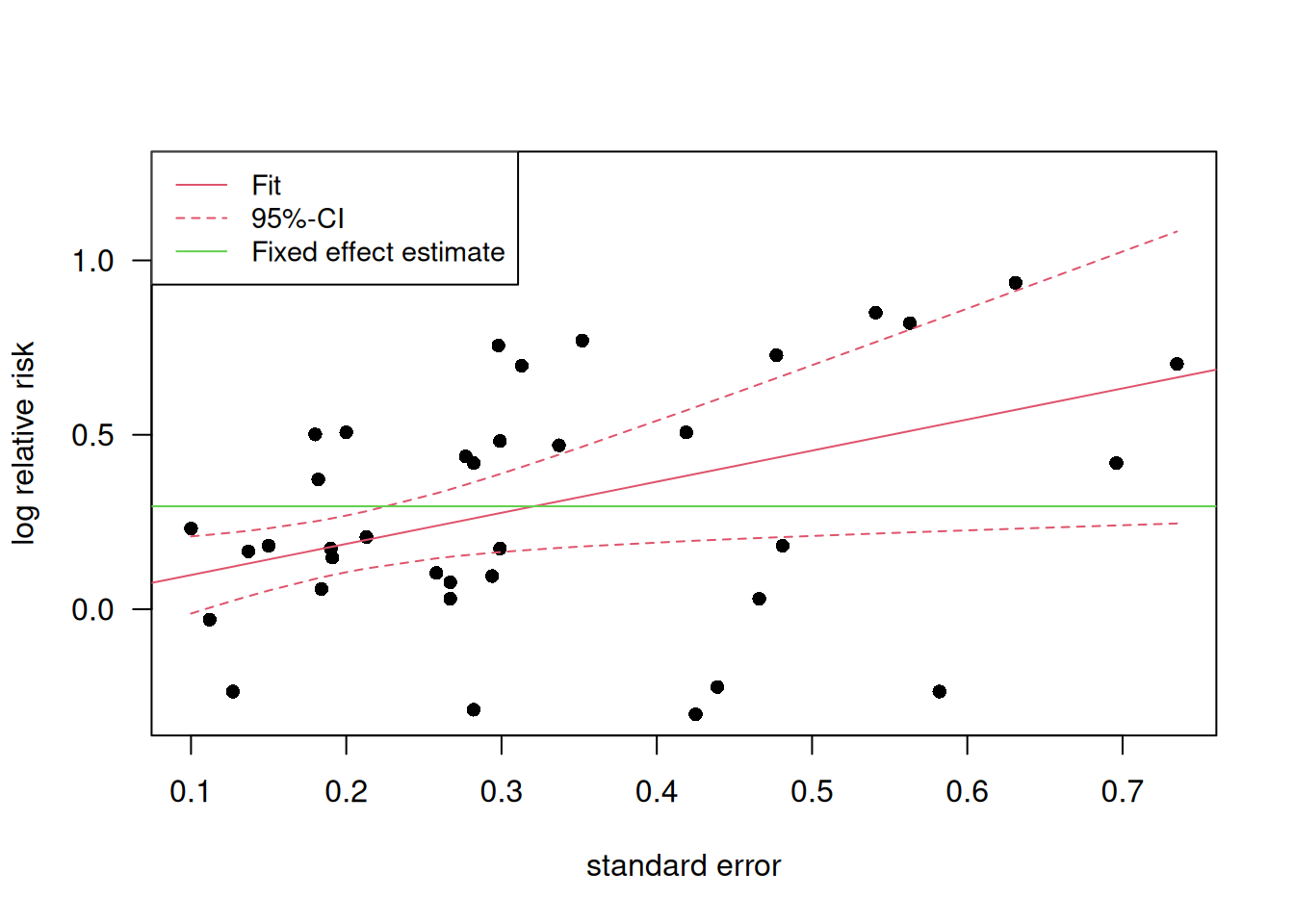
Figure 15.8: Visualization of Egger’s weighted regression in the passive smoking example.
Egger’s test in R:
## Linear regression test of funnel plot asymmetry
##
## Test result: t = 2.37, df = 35, p-value = 0.0236
## Bias estimate: 0.8915 (SE = 0.3768)
##
## Details:
## - multiplicative residual heterogeneity variance (tau^2 = 1.1704)
## - predictor: standard error
## - weight:    inverse variance
## - reference: Egger et al. (1997), BMJ
Limit meta-analysis
The aim of a limit meta-analysis is to compute a bias-adjusted overall effect estimate by extrapolating the weighted regression to \(s_i \to 0\).
A limit meta-analysis can be performed in R
using the function metasens::limitmeta().
For Example 15.3, this gives:
## Result of limit meta-analysis:
##
##  Random effects model                   95%-CI    z
##     Adjusted estimate 0.0982 [-0.0574; 0.2538] 1.24
##   Unadjusted estimate 0.2183 [ 0.1222; 0.3143] 4.45
##      pval
##    0.2160
##  < 0.0001
##
## Quantifying heterogeneity:
## tau^2 = 0.0220; I^2 = 24.2% [0.0%; 49.8%]; G^2 = 95.0%
##
## Test of heterogeneity:
##      Q d.f. p-value
##  47.52   36  0.0949
##
## Test of small-study effects:
##   Q-Q' d.f. p-value
##   6.55    1  0.0105
##
## Test of residual heterogeneity beyond small-study effects:
##     Q' d.f. p-value
##  40.96   35  0.2252
##
## Details on adjustment method:
## - expectation (beta0)