Chapter 9 Survival analysis
A common form of data in clinical trials is survival (time to event) data. Survival outcomes can often be considered as continuous, but are usually quite skewed. Moreover, the issue of censoring requires special techniques for statistical analysis.
9.1 Analysis of survival outcomes
9.1.1 Censoring
A survival time \(T\) is called (right-)censored, if it is known that the individual has survived up to time \(T\), but whose survival status past that point is not known. For example, the study might be finished before all patients have died, a patient might decide to withdraw from the study or a patient might die from some other reason, for example in a car crash.
A central assumption in survival analysis is that the censoring time is independent of the survival time (non-informative censoring).
Example 9.1 The Chemotherapy study (Huguenin et al, 2004) is a randomized study to compare two treatments for head and neck cancer on \(224\) patients: Combination of radiotherapy and chemotherapy (RT+CT) (\(n=112\)) versus radiotherapy alone (RT) (\(n=112\)). The primary outcome is survival time (in years) from start of treatment. Figure 9.1 shows data for the survival times of the first 10 patients. The survival time is measured from the start of treatment (starting point \(0\)) and it ends if a patient either dies or is censored.
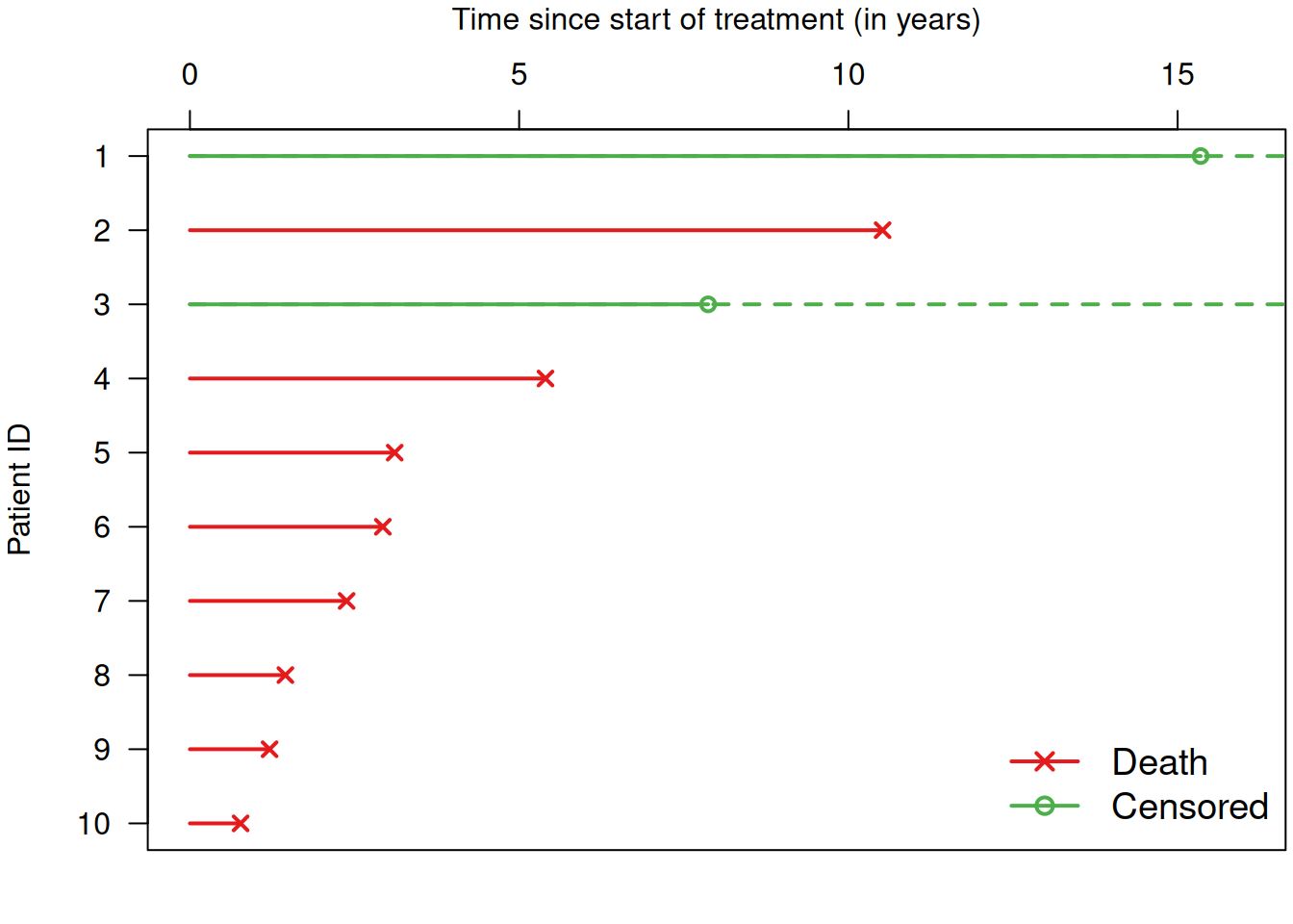
Figure 9.1: Survival times for a selection of patients from Example 9.1.
Table 9.1 shows a selection of variables for the first five
patients. The notion of overall of survival (OS) denotes survival without any further
conditions (in contrast to, e.g., progression free survival).
In this example, OS is the survival time in years and the \(+\) stands for
“censored”. The format of the variable OS (with \(+\) for censored) is the output
of the R function survival::Surv().
| ID | Sex | Age | Treatment | LK | Stage | PS | OS |
|---|---|---|---|---|---|---|---|
| 1 | Female | 57.4 | RT+CT | 2c | 4 | 1 | 15.3+ |
| 2 | Male | 66.9 | RT+CT | 0 | 3 | 1 | 10.5 |
| 3 | Male | 68.3 | RT+CT | 0 | 3 | 1 | 7.9+ |
| 4 | Male | 51.6 | RT | 0 | 2 | 0 | 5.4 |
| 5 | Male | 38.8 | RT | 2c | 4 | 0 | 3.1 |
9.1.2 Survival function and curve
The survival function
\[\begin{equation*} S(t) = \Pr(T > t) \end{equation*}\]
gives the probability of survival at least up to time \(t\). The survival curve is a plot of \(S(t)\) versus \(t\), see Figure 9.2.
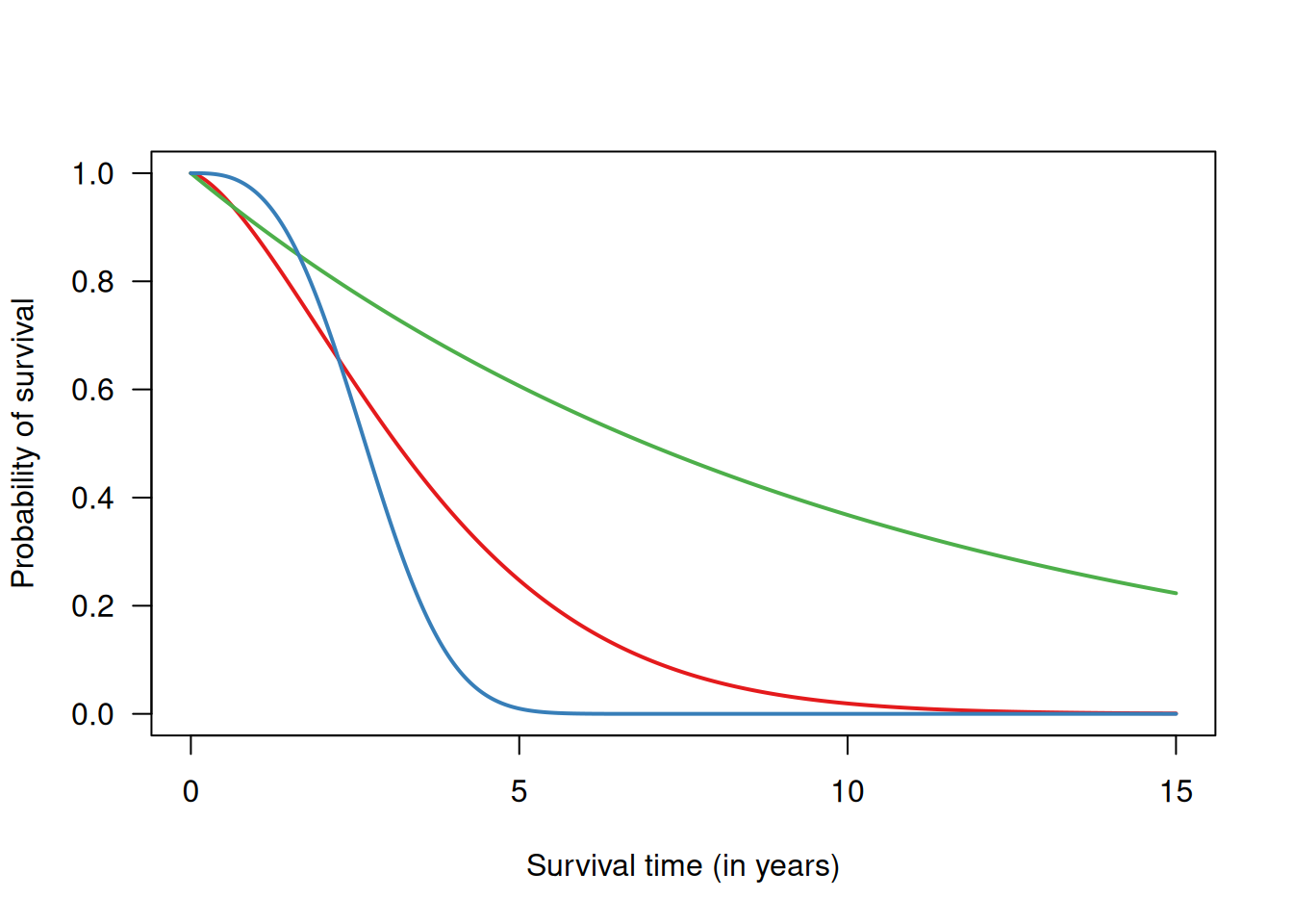
Figure 9.2: Examples of survival curves for three different survival functions.
Life table method
The life table method is a classical approach to estimate the survival function \(S(t)\). It is based on a partition of the time axis into time intervals \(i=1,\ldots,I\) of typically equal length. The risk of death \(r_i\) in interval \(i\) is estimated as
\[\begin{equation*} \hat r_i = \frac{\mbox{# patients which died in interval $i$}}{\mbox{# patients at risk in interval $i$}} = \frac{d_i}{n_i} \end{equation*}\]
By convention, observations censored in interval \(i\) contribute half to the number of patients at risk. Note that the denominator \(n_i\) is monotonically decreasing as a function of time.
The survival function is then estimated as
\[\begin{equation*} \hat S(i) = \prod_{t=1} ^i(1 - \hat r_t) = (1 - \hat r_1) \times \ldots \times (1 - \hat r_i). \end{equation*}\]
Wald confidence intervals can be calculated for \(\hat S(i)\), \(\log \hat S(i)\) or \(\log \{-\log \hat S(i)\}\) with appropriate back-transformation. The corresponding standard errors can be found in textbooks, e.g. Collett (2003) (Section 2.2).
Example 9.1 (continued) Table 9.2 shows the estimated survival function (values for each interval/year) in the RT+CT group from Example 9.1. Figure 9.3 shows the estimated survival curve with 95% confidence intervals for every year (in red).
| Interval (year) | # patients at beginning of interval | # deaths during interval | # censored | # patients at risk | \(r_i\) | \(1-r_i\) | \(\hat S(i)\) |
| 1 | 112 | 25 | 0 | 112 | 0.22 | 0.78 | 0.78 |
| 2 | 87 | 14 | 1 | 86.5 | 0.16 | 0.84 | 0.65 |
| 3 | 72 | 10 | 1 | 71.5 | 0.14 | 0.86 | 0.56 |
| 4 | 61 | 8 | 1 | 60.5 | 0.13 | 0.87 | 0.49 |
| 5 | 52 | 4 | 4 | 50 | 0.08 | 0.92 | 0.45 |
| 6 | 44 | 3 | 5 | 41.5 | 0.07 | 0.93 | 0.41 |
| 7 | 36 | 4 | 3 | 34.5 | 0.12 | 0.88 | 0.37 |
| 8 | 29 | 4 | 3 | 27.5 | 0.15 | 0.85 | 0.31 |
| 9 | 22 | 1 | 3 | 20.5 | 0.05 | 0.95 | 0.3 |
| 10 | 18 | 1 | 5 | 15.5 | 0.06 | 0.94 | 0.28 |
| 11 | 12 | 2 | 0 | 12 | 0.17 | 0.83 | 0.23 |
| 12 | 10 | 0 | 1 | 9.5 | 0 | 1 | 0.23 |
| 13 | 9 | 2 | 2 | 8 | 0.25 | 0.75 | 0.17 |
| 14 | 5 | 1 | 2 | 4 | 0.25 | 0.75 | 0.13 |
| 15 | 2 | 0 | 1 | 1.5 | 0 | 1 | 0.13 |
| 16 | 1 | 0 | 1 | 0.5 | 0 | 1 | 0.13 |
Kaplan-Meier estimate of the survival function
In many studies, the exact follow-up time for each individual is known. Aggregation in arbitrary time intervals can then be avoided. The Kaplan-Meier estimate of the survival function uses intervals which contain only up to one event, so \(d_i \in \{0, 1\}\) (if there are no ties). Application of the life table method to these intervals yields the Kaplan-Meier estimate, a step function with jumps of relative size \[ 1/\mbox{number of subjects at risk} \] at the time of each event.
There are some critical assumptions in Kaplan-Meier estimation (Bland and Altman, 1998): First, at any time, patients who are censored have the same survival prospects as those who continue to be followed. If censoring is related to survival for some patients, the estimated survival probabilities would be biased. Secondly, survival probabilities are the same for subjects recruited early and late in the study. In a long term study, the case mix may change over the period of recruitment, or there may be an innovation in ancillary treatment. Last, the event happens at the time specified. This could be a problem, for example, if the event were recurrence of a tumor which would be detected at a regular examination (interval censoring).
The results of a survival analysis depend upon the choice of time scale: time since study entry (i.e. randomisation in RCTs), calendar time, or age. For example, consider the following dataset:
##    Subject Sex  DateEntry AgeEntry   DateExit AgeExit Event
## 1        1   F 1965-06-13     29.3 1989-12-31    53.8     0
## 2        2   M 1972-10-23     25.2 1989-12-31    42.4     0
## 3        3   M 1959-03-03     22.1 1989-12-31    52.8     0
## 4        4   F 1967-10-10     32.2 1989-12-31    54.4     0
## 5        5   M 1960-01-02     33.1 1979-07-04    52.6     1
## 6        6   M 1975-01-09     42.1 1989-12-31    57.1     0
## 7        7   F 1953-08-05     35.2 1968-10-03    50.4     1
## 8        8   M 1969-10-10     27.0 1989-12-31    47.2     0
## 9        9   M 1972-03-02     44.8 1989-12-31    62.7     0
## 10      10   F 1970-11-01     51.5 1989-12-31    70.6     0
With this dataset, the three time scales look as follows:
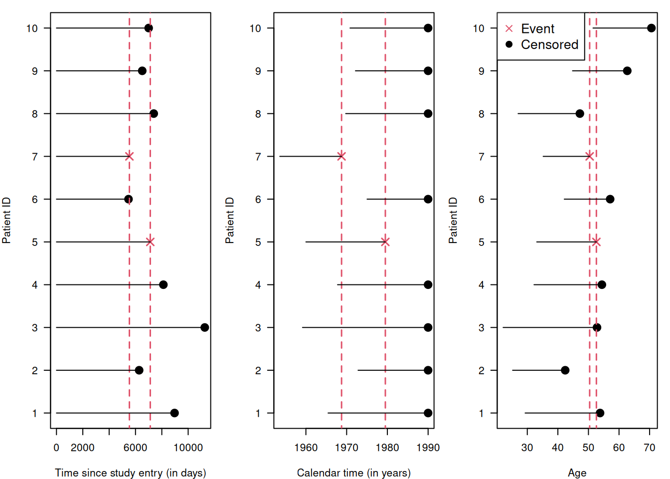
| Time scale | Risk set at first event | Risk set at second event |
|---|---|---|
| Time since study entry | {1, 2, 3, 4, 5, 7, 8, 9, 10} | {1, 3, 4, 5, 8} |
| Calendar time | {1, 3, 4, 5, 7} | {1, 2, 3, 4, 5, 6, 8, 9, 10} |
| Age | {1, 3, 4, 5, 6, 7, 9} | {1, 3, 4, 5, 6, 9, 10} |
The risk set depends on the time scale. Then how do we select a time scale? Usually, the time scale with the strongest relationship to the event rate is used. In RCTs, survival is usually analysed in relation to the time since randomisation. An additional time scale can be incorporated as a covariate. For example, one can adjust for the age of the subjects by including age at diagnosis (which is fixed for every subject) in a short follow-up, and by including age itself as a time-varying covariate in a long follow-up.
Example 9.1 (continued) Figure 9.3 compares the Kaplan-Meier estimate of
the survival curve in Example 9.1 for the RT+CT group
to the estimate obtained with the life table method
using yearly intervals.
The Kaplan-Meier estimate can be calculated and plotted with the following R code.
The option conf.int = TRUE shows a dotted confidence band and the option
mark.time = TRUE would show censoring events (see Figure 9.5).
sakk.surv <- survfit(Surv(os, death) ~ 1, data = sakk.rtct,
                     conf.type = "log-log")
plot(sakk.surv, conf.int = TRUE, mark.time = FALSE, lwd = 2,
     col = col.blue, log = FALSE, xlab = "Survival time (in years)",
     ylab = "Survival probability", xlim = c(0, Imax))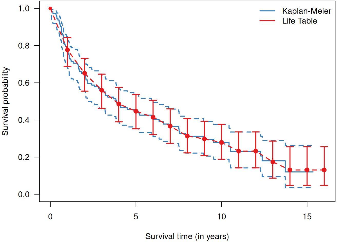
Figure 9.3: Comparison of Kaplan-Meier method (blue) with life table method (red, with yearly 95% confidence intervals) to estimate the survival curve in the RT+CT group from Example 9.1.
With survminer::ggsurvplot, a Kaplan-Meier estimate with additional risk
table can be obtained as shown in Figure 9.4.
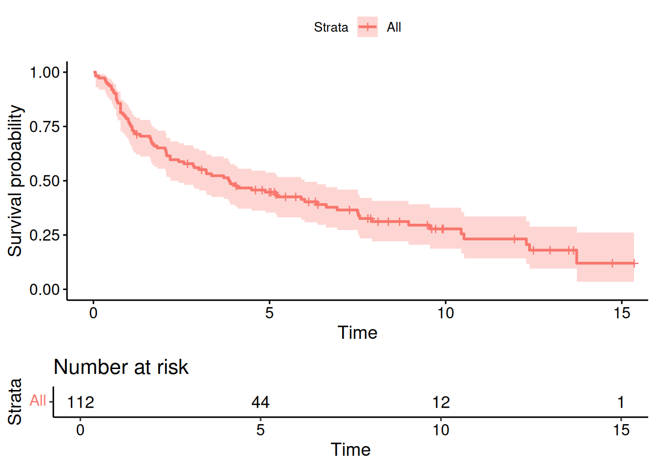
Figure 9.4: Kaplan-Meier estimate of the survival curve in the RT+CT group from Example 9.1, with risk table.
Based on the Kaplan-Meier curve we can now compute survival probabilities with confidence interval, for example at 5 years:
## Call: survfit(formula = Surv(os, death) ~ 1, data = sakk.rtct, conf.type = "log-log")
##
##  time n.risk n.event survival std.err lower 95% CI
##     5     44      61    0.447  0.0476        0.353
##  upper 95% CI
##         0.538
It is important to be careful with censored data. Censored observations cannot be simply ignored, i.e. excluded, and they cannot be treated as non-censored. Doing so would lead to biased estimation of the survival function as illustrated in Figure 9.5. Excluding censored observations means losing data on patients without events, so will underestimate the survival curve. Treating them as non-censored, i.e. as death events, also leads to underestimation of the survival curve.
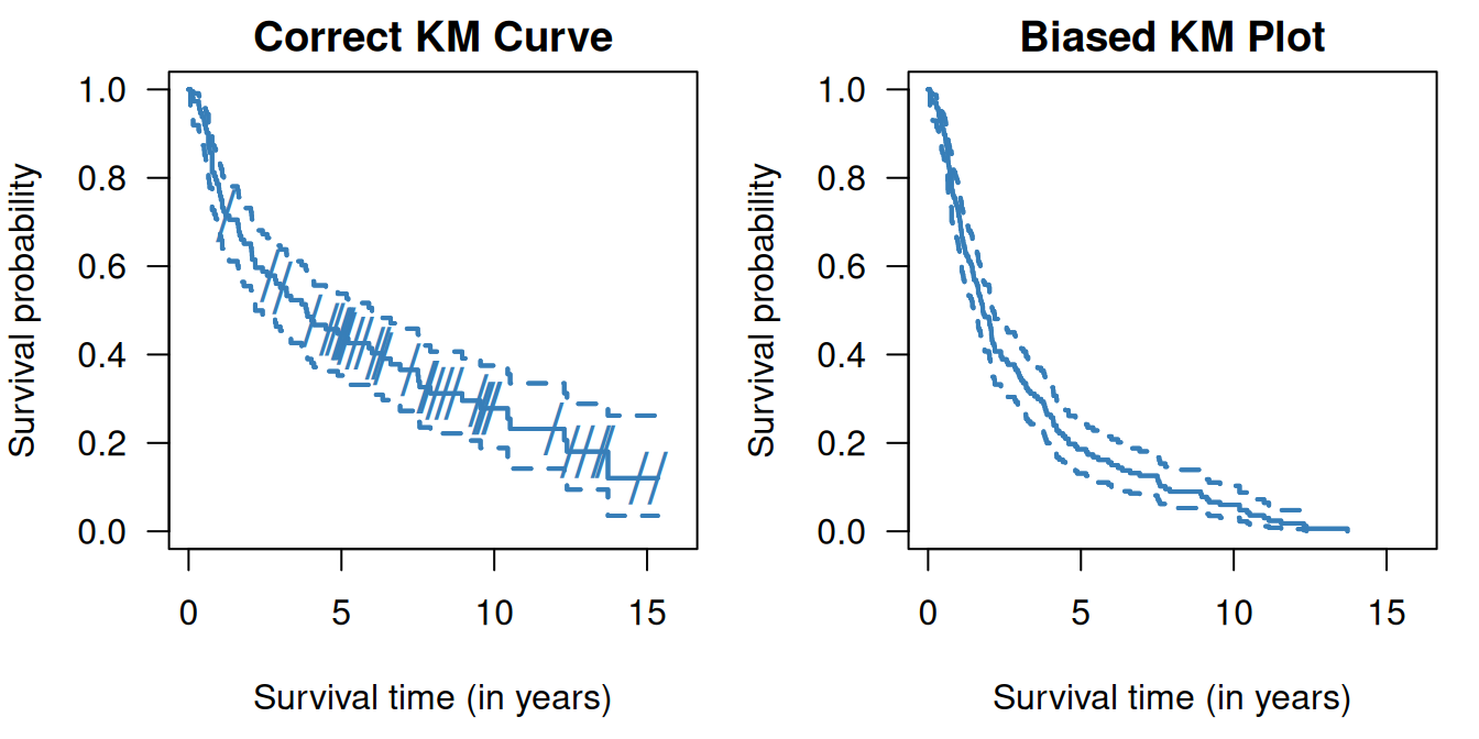
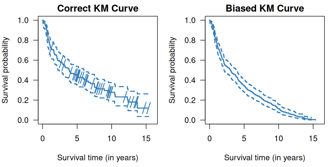
Figure 9.5: Kaplan-Meier curves in the RT+CT group from Example 9.1 where censored observations are ignored (top right) and where censored observations are treated as non-censored (bottom right). On the left side (top and bottom) the correct Kaplan-Meier estimate is shown, the dashes indicate censoring events.
9.1.3 Median survival time
The median survival time \(t_{\small{\mbox{Med}}}\) (and other quantiles) can be easily read off the Kaplan-Meier estimate. A confidence interval for the \(t_{\small{\mbox{Med}}}\) can also be derived in this way. The “square-and-add” method, see Appendix A.2.3, can be used to compute a confidence interval for the difference in median survival time between two groups.
Example 9.1 (continued) Figure 9.6 is a graphical illustration of the median survival time in the RT+CT group from Example 9.1.
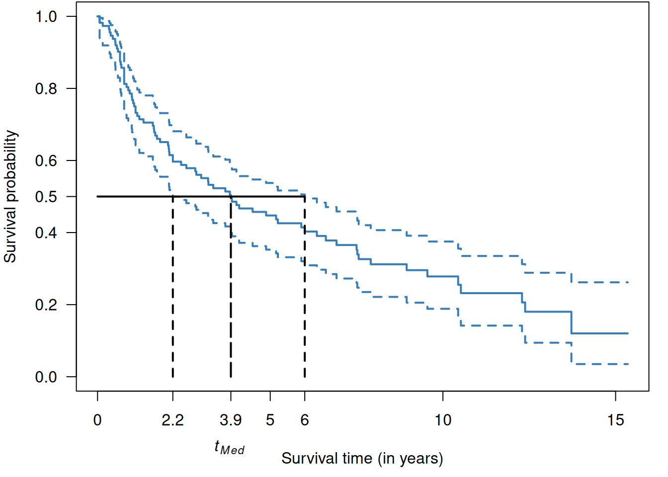
Figure 9.6: Median survival time in the RT+CT group from Example 9.1.
| \(t_{\small{\mbox{Med}}}\) | 95%-CI | |||
|---|---|---|---|---|
| \(n\) | Number of Deaths | (in years) | (in years) | |
| RT + CT | 112 | 79 | 3.9 | from 2.2 to 6.0 |
| RT | 112 | 88 | 2.4 | from 1.8 to 3.8 |
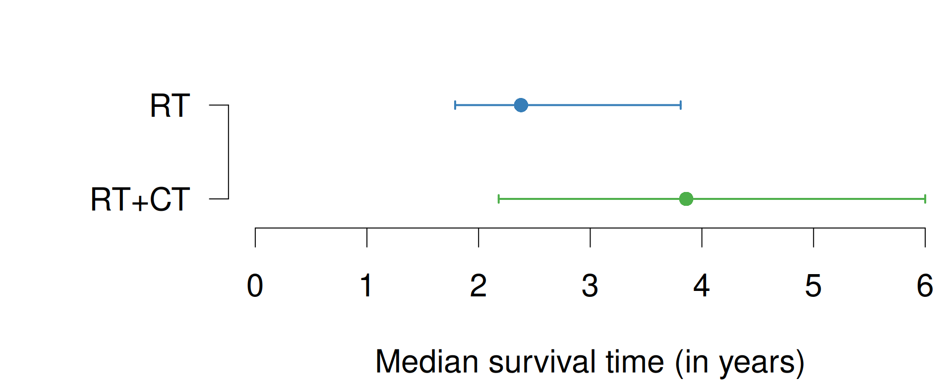
Figure 9.7: Median survival times with 95% confidence intervals of RT and RT+CT groups from Example 9.1.
The median survival time in the two groups with their respective CI are shown in Table 9.3 and graphically in Figure 9.7.
The difference in median survival time is 1.5 years
(95%-CI: from \(-0.7\) to \(3.7\) years) and is
computed with the R function biostatUZH::confIntSquareAdd():
biostatUZH::confIntSquareAdd(theta1 = 3.9, lower1 = 2.2, upper1 = 6,
                             theta2 = 2.4, lower2 = 1.8, upper2 = 3.8)
## $difference
## [1] 1.5
##
## $CI
## lower upper
## 1 -0.7022716 3.6840339.2 Comparison of survival curves
One has to be careful about what groups to compare. Breslow’s first rule of survival analysis states that: “Selection into the study cohort, or into subgroups to be compared in the analysis, must not depend on events that occur after the start of follow-up”. Survival by tumor response analysis in oncology is an example that leads to biased estimates of the survival distributions, invalid statistical tests, and misleading conclusions. This bias results from the fact that responders must live long enough for response to be observed; there is no such requirement for non-responders, see Anderson et al (2008). Another example where Breslow’s rule is violated is a study reporting that Oscar winners live longer (Redelmeier and Singh, 2001). As other scientists have noticed, this study was subject to survival bias or immortal time bias (Sylvestre et al, 2006).
We now discuss how survival curves can be compared between groups.
For example, the survival curves of the RT and RT+CT groups are shown in Figure 9.8. Later, we show how to generate
such a plot with the Rfunction ggminer::ggsurvplot. In Section 9.4 we will describe methods to incorporate time-varying covariates in the analysis to avoid immortal time bias.
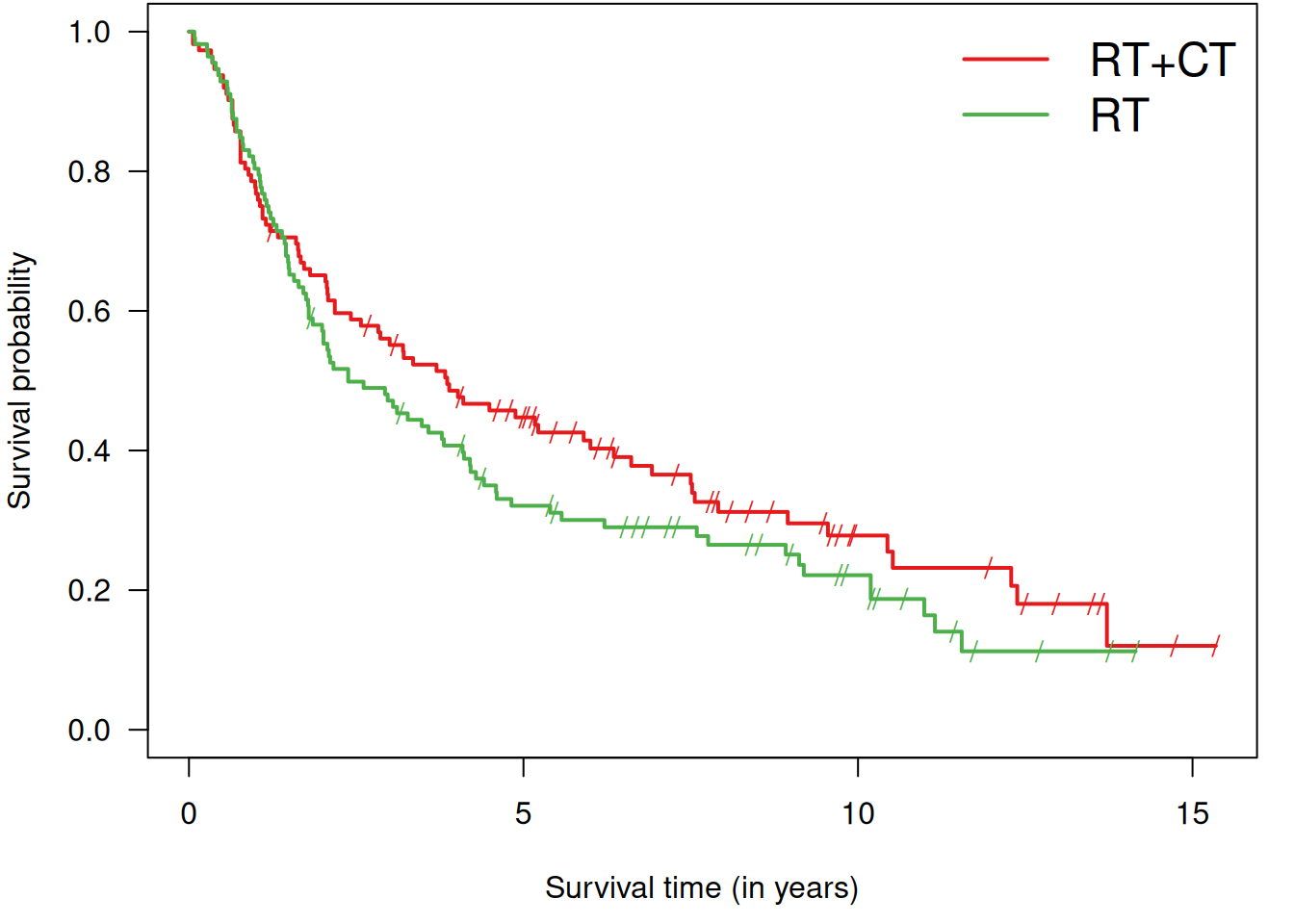
Figure 9.8: Kaplan-Meier curves for both groups in Example 9.1.
9.2.1 Log-rank test
The log-rank test, also called Mantel-Cox test, quantifies the evidence against the null hypothesis of equal survival curves \(S_A(t) = S_B(t)\), in groups A and B, for all times \(t\) with a \(P\)-value. The method compares the observed number of events with the corresponding expected number of events (under the null hypothesis \(H_0\)) in each group.
## Call:
## survdiff(formula = Surv(time, death) ~ treat, data = sakk)
##
##               N Observed Expected (O-E)^2/E (O-E)^2/V
## treat=RT+CT 112       79     87.5     0.822      1.74
## treat=RT    112       88     79.5     0.904      1.74
##
##  Chisq= 1.7  on 1 degrees of freedom, p= 0.2
The two survival curves can be shown in one plot using the following code, see Figure 9.9:
sakk.surv1 <- survfit(Surv(time, death) ~ treat, data = sakk, conf.type = "log-log")
ggsurvplot(sakk.surv1, risk.table = TRUE, conf.int = TRUE, pval = TRUE)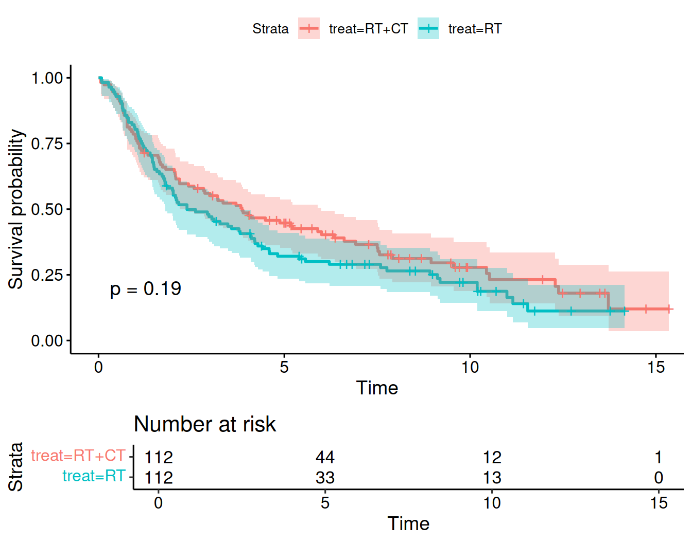
Figure 9.9: Kaplan-Meier curves for both groups in Example 9.1 obtained with ggsurvplot.
9.2.2 Hazard function
The mortality rate can also be used to describe the risk of death in a certain interval: \[\begin{eqnarray*} \frac{\mbox{Death risk in interval}}{\mbox{Length of interval}}. \end{eqnarray*}\]
The mortality rate is conditional on having survived up to the interval of interest. The hazard function is obtained by making the length of the intervals very small:
\[\begin{equation*} h(t)= \lim\limits_{h \rightarrow 0} \frac{\operatorname{\mathsf{Pr}}(t < T < t+h \,\vert\,T>t)}{h}. \end{equation*}\]
The hazard function and the survival function have a one-to-one relationship:
\[\begin{equation*} S(t) = \exp\left(- \int_0^t h(u) du \right). \end{equation*}\] This implies that the cumulative hazard function \(H(t)\) is directly related to the survival function: \[\begin{equation*} H(t) = \int_0^t h(u) du = - \log S(t). \end{equation*}\]
Figure 9.10 shows the survival and hazard functions for a constant hazard rate (\(\mbox{HR} = 2\), top) and for an increasing hazard rate (bottom).
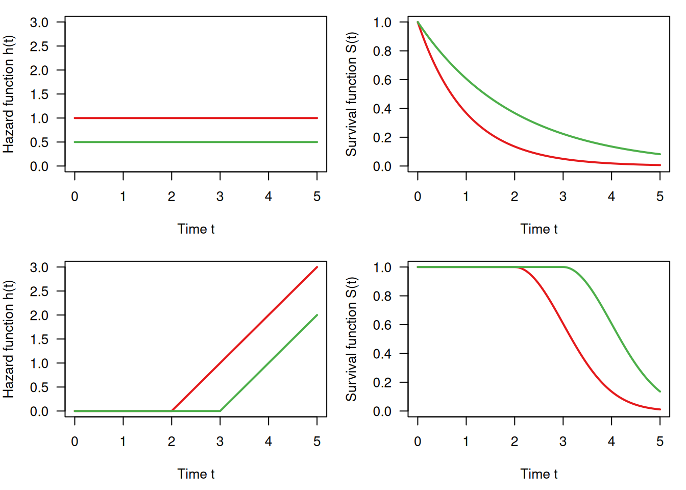
Figure 9.10: Survival function and hazard function: constant hazard (top) and non-linearly increasing (bottom)
9.2.3 Hazard ratio
Let \(h_A(t)\) and \(h_B(t)\) denote the hazard functions in groups A and B. The proportional hazards assumption implies a time-constant hazard ratio
\[\begin{equation*} \mbox{HR} = {h_A(t)}/{h_B(t)}. \end{equation*}\]
The hazard ratio can be interpreted as
- (instantaneous) relative risk at any time \(t>0\):
\[\begin{equation*} \mbox{HR} = \frac{h_A(t)}{h_B(t)}\approx \frac{{\operatorname{\mathsf{Pr}}(t < T_A < t+h \,\vert\,T_A>t)}/{h}}{{\operatorname{\mathsf{Pr}}(t < T_B < t+h \,\vert\,T_B>t)}/{h}} \equiv \frac{{\operatorname{\mathsf{Pr}}(t < T_A < t+h \,\vert\,T_A>t)}}{{\operatorname{\mathsf{Pr}}(t < T_B < t+h \,\vert\,T_B>t)}} \end{equation*}\]
- ratio of the cumulative hazard functions at any time \(t>0\):
\[\begin{equation*} \mbox{HR} = \frac{H_A(t)}{H_B(t)} = \frac{\log S_A(t)}{\log S_B(t)} \end{equation*}\] so the survival function in group A is the survival function in group B to the power of HR: \[\begin{equation*} S_A(t) = S_B(t)^{\scriptsize \mbox{HR}}. \end{equation*}\]
The hazard ratio can be calculated from the output of the log-rank test as the ratio of the relative event rates (observed/expected) in the two groups. Only the observed and expected number of cases are required. This simple estimate is known as the Pike hazard ratio estimate and has been shown to slightly underestimate larger effects. It has only little bias for hazard rates typically observed in clinical trials.
## [1] 79 88## [1] 87.48016 79.51984## [1] 0.9030619 1.1066420HR <- EventRates[2]/EventRates[1]
SElogHR <- sqrt(sum(1/expected))
printWaldCI(log(HR), SElogHR, FUN = exp)## Effect 95% Confidence Interval P-value
## [1,] 1.225 from 0.904 to 1.660 0.19In the example, the hazard ratio turns out to be \(\mbox{HR}=1.225\).
The Cox model
The (semiparametric) Cox model assumes that the hazard function \(h_i(t)\) of individual \(i\) with explanatory variables \(\boldsymbol{ x}_i\) has the form
\[\begin{equation*} h_i(t; \boldsymbol{ x}_i) = \exp(\boldsymbol{ x}_i^{\top} \boldsymbol{ \beta}) \cdot h_0(t), \end{equation*}\]
where \(h_0(t)\) is the baseline hazard function. Ratios of hazard functions are time-constant:
\[\begin{equation*} \frac{h_i(t; \boldsymbol{ x}_i)}{h_j(t; \boldsymbol{ x}_j)} = \frac{\exp(\boldsymbol{ x}_i^{\top} \boldsymbol{ \beta})} {\exp(\boldsymbol{ x}_j^{\top} \boldsymbol{ \beta})}, \end{equation*}\]
i.e. we have proportional hazards. A profile likelihood approach allows to estimate the log hazard ratios \(\boldsymbol{ \beta}\), no matter which form \(h_0(t)\) has. To estimate the hazard ratio, we use Cox-Regression as in the following example.
Example 9.1 (continued) Cox regression in Example 9.1:
| Hazard Ratio | 95%-confidence interval | \(p\)-value |
|---|---|---|
| 1.23 | from 0.90 to 1.66 | 0.19 |
The comparison RT vs. RT+CT gives \(\mbox{HR}=1.23\) with relatively large confidence interval, very close to the one obtained with Pike’s method based on the log-rank test. There is no evidence for a treatment effect (\(p=0.19\)).
Adjusting in survival analysis
There may be differences between treatment groups in important baseline characteristics. Table 9.5 shows the distribution of gender in the two treatment groups in Example 9.1, which is surprisingly unbalanced (percentage female 10% resp. 21%). It is recommended to adjust the treatment effect for potential confounders at baseline, which can be done with Cox regression.
| RT + CT | RT | |
|---|---|---|
| F | 11 | 23 |
| M | 101 | 89 |
Example 9.1 (continued) Adjusting for baseline values with Cox regression in Example 9.1:
| Hazard Ratio | 95%-confidence interval | \(p\)-value |
|---|---|---|
| 1.26 | from 0.92 to 1.71 | 0.14 |
| 0.81 | from 0.52 to 1.26 | 0.34 |
The adjusted hazard of death (instantaneous death risk) is increased by \(26\)% for RT relative to RT + CT (\(p=0.14\)). Women have a \(19\)% reduced hazard of death (\(p=0.34\)) compared to men. However, there is no evidence for a difference in both cases as the corresponding \(P\)-values are large.
9.3 Sample size in survival studies
Both the number of events and the total number of patients are of interest in a survival study.
9.3.1 Total number of events
There is a simple formula for the required total number of events (Collett, 2003, chap. 10)):
\[\begin{equation*} d = \frac{ 4 (u + v)^2}{ \Delta^2}, \end{equation*}\] where \(\Delta\) is the log hazard ratio to be detected, and \(u\), \(v\) are the same as the ones defined in Section 5.2.
The number of events can be calculated with
the Rfunction biostatUZH::survEvents():
## [1] 2279.3.2 Total number of patients
The required total number of patients \(n\) can be found from
\[\begin{equation*} n = d / \Pr(\mbox{event}), \end{equation*}\]
where \(\Pr(\mbox{event})\) is calculated based on the assumed survival functions in the two groups and assumptions on the accrual period \(a\) and the follow-up period \(f\).
Example 9.2 The survival probability of females in the lung cancer data from Loprinzi et al (1994) is shown in Figure 9.11.
data(cancer, package = "survival")
cancer.female <- subset(cancer, sex == 2)
survObj <- Surv(time = cancer.female$time,
                event = (cancer.female$status == 2))
fit <- survfit(survObj ~ 1)
ggsurvplot(fit, data = cancer.female)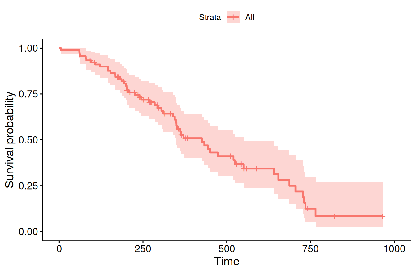
Figure 9.11: Kaplan-Meier estimate of the survival curve of females in the lung cancer data from Loprinzi et al (1994).
In order to detect a hazard ratio of \(0.65\) with power 90% for accrual and follow-up time period of 400 days, 379 patients are required:
res <- sampleSizeSurvival(HR = 0.65, power=.9, sig.level=0.05,
                          a.length = 400, f.length = 400,
                          dist = "non-parametric", survfit.ref = fit)
print(t(res))
## n HR power sig.level alternative distribution
## [1,] 379 0.65 0.9 0.05 "two.sided" "non-parametric"
## PrEvent Events
## [1,] 0.5996061 227Instead of a non-parametric fit of the survival curves, the function can also be given a parametric input for the survival curves such as a Weibull or exponential distribution with specified parameters.
9.4 Time-varying explanatory variables
Time-varying explanatory variables, e.g. exposure yes/no, can be dealt with by
- splitting the follow-up of each patient into parts with constant covariate values and
- treating the parts as distinct subjects.
This approach requires allowance for late entries in the analysis, which is the case in R. The approach is valid if changes in explanatory variables are unrelated to the underlying risk of failure. We will now see two examples of time-dependent analyses.
Example 9.3 The PBC study is about treatment of primary biliary cirrhosis (PBC) of the liver. We will use the first 312 cases in this dataset from the survival package since they participated in the randomized trial and contain largely complete data. The status at endpoint can be 0 = censored, 1 = transplant or 2 = dead.
library(survival)
data("pbc")
sel <- c("id", "time", "status", "trt", "age", "sex", "bili", "protime")
## baseline data
head(pbc[,sel])
## id time status trt age sex bili protime
## 1 1 400 2 1 58.76523 f 14.5 12.2
## 2 2 4500 0 1 56.44627 f 1.1 10.6
## 3 3 1012 2 1 70.07255 m 1.4 12.0
## 4 4 1925 2 1 54.74059 f 1.8 10.3
## 5 5 1504 1 2 38.10541 f 3.4 10.9
## 6 6 2503 2 2 66.25873 f 0.8 11.0Variables bili and protime are time-dependent measurements. The baseline data shown above, in contrast, only include baseline measurements of these covariates that have multiple measurements over time.
sel <- c("id", "futime", "status", "trt", "age", "sex", "day", "bili", "protime")
head(pbcseq[,sel], 14)
## id futime status trt age sex day bili protime
## 1 1 400 2 1 58.76523 f 0 14.5 12.2
## 2 1 400 2 1 58.76523 f 192 21.3 11.2
## 3 2 5169 0 1 56.44627 f 0 1.1 10.6
## 4 2 5169 0 1 56.44627 f 182 0.8 11.0
## 5 2 5169 0 1 56.44627 f 365 1.0 11.6
## 6 2 5169 0 1 56.44627 f 768 1.9 10.6
## 7 2 5169 0 1 56.44627 f 1790 2.6 11.3
## 8 2 5169 0 1 56.44627 f 2151 3.6 11.5
## 9 2 5169 0 1 56.44627 f 2515 4.2 11.5
## 10 2 5169 0 1 56.44627 f 2882 3.6 11.5
## 11 2 5169 0 1 56.44627 f 3226 4.6 11.5
## 12 3 1012 2 1 70.07255 m 0 1.4 12.0
## 13 3 1012 2 1 70.07255 m 176 1.1 12.0
## 14 3 1012 2 1 70.07255 m 364 1.5 12.0In a baseline analysis (including only baseline measurements), first without and then with adjustment for covariates, we obtain the following results:
## baseline fit for first 312 patients
fit0 <- coxph(Surv(time, status == 2) ~ trt,
              data = pbc, subset = (id <= 312))
fit1 <- coxph(Surv(time, status == 2) ~ trt + log(bili) + log(protime),
data = pbc, subset = (id <= 312))| Hazard Ratio | 95%-confidence interval | \(p\)-value |
|---|---|---|
| 0.94 | from 0.66 to 1.34 | 0.75 |
| Hazard Ratio | 95%-confidence interval | \(p\)-value |
|---|---|---|
| 0.91 | from 0.64 to 1.29 | 0.59 |
| 2.64 | from 2.20 to 3.17 | < 0.0001 |
| 78.76 | from 12.60 to 492.44 | < 0.0001 |
A time-dependent analysis includes all measurements of the covariates. First, we need to prepare the data accordingly. The data preparation below is adopted from vignette timedep.pdf in package survival. It therefore also contains the variables ascites, albumin and alk.phos that are not used in the following analysis.
temp <- subset(pbc, id <= 312, select = c(id:sex, stage)) # baseline
pbc2 <- tmerge(temp, temp, id = id, death = event(time, status)) #set range
pbc2 <- tmerge(pbc2, pbcseq, id = id, bili = tdc(day, bili),
               protime = tdc(day, protime))
head(pbc2)
## id time status trt age sex stage tstart tstop death
## 1 1 400 2 1 58.76523 f 4 0 192 0
## 2 1 400 2 1 58.76523 f 4 192 400 2
## 3 2 4500 0 1 56.44627 f 3 0 182 0
## 4 2 4500 0 1 56.44627 f 3 182 365 0
## 5 2 4500 0 1 56.44627 f 3 365 768 0
## 6 2 4500 0 1 56.44627 f 3 768 1790 0
## bili protime
## 1 14.5 12.2
## 2 21.3 11.2
## 3 1.1 10.6
## 4 0.8 11.0
## 5 1.0 11.6
## 6 1.9 10.6## time-dependent fit
fit2 <- coxph(Surv(tstart, tstop, death == 2) ~ trt + log(bili) +
log(protime), data = pbc2)| Hazard Ratio | 95%-confidence interval | \(p\)-value |
|---|---|---|
| 0.94 | from 0.65 to 1.34 | 0.72 |
| 3.46 | from 2.86 to 4.19 | < 0.0001 |
| 53.39 | from 22.78 to 125.14 | < 0.0001 |
The analysis reveals that – after taking into account adjustments
for time-varying covariates – the effect of trt is weaker with a HR of
0.94 rather than 0.91 and a larger \(p\)-value.
Example 9.4 Survival by tumor response revisited, see Section 9.2. This example is about survival in patients with advanced lung cancer shown in Figure 9.12.
KMfit <- survfit(Surv(time/365.25, status) ~ 1, data = lung)
ggsurvplot(KMfit, xlab = "Years post diagnosis", ylab = "Survival",
           conf.int = TRUE)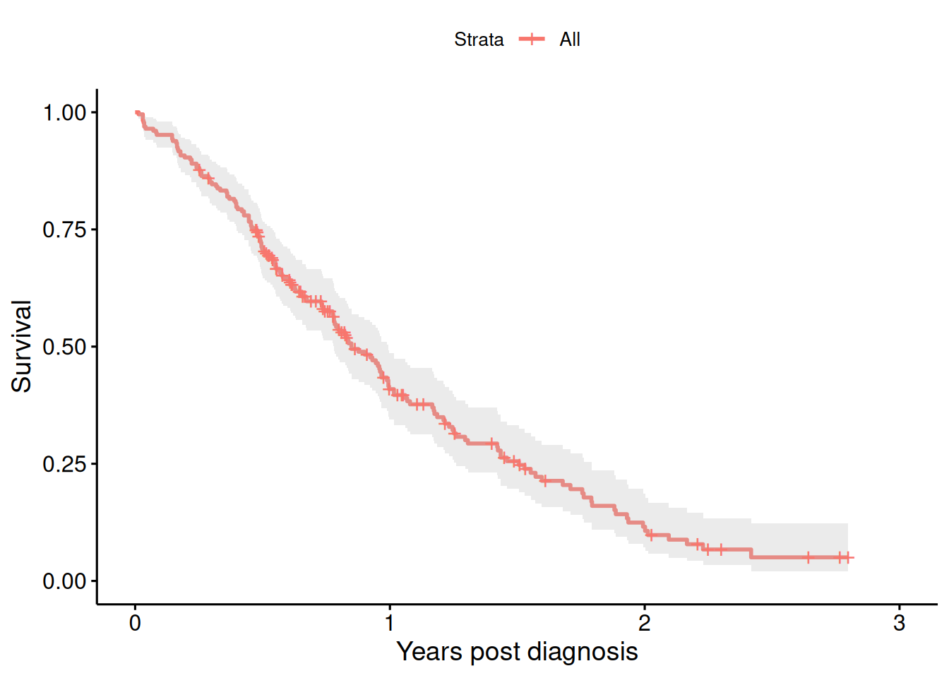
Figure 9.12: Kaplan-Meier estimate of the survival curve of patients with advanced lung cancer.
We now randomly generate tumor “responders” with a probability of \(0.05\) to become a responder at every month within the first year.
##      0 1 2 3 4 5 6 7 8 9 10 11 12
## [1,] 0 0 0 0 0 0 0 0 0 0  0 NA NA
## [2,] 0 0 0 0 0 1 1 1 1 1  1  1  1
## [3,] 0 0 0 0 0 0 1 1 1 1 1 1 1## responder
## FALSE TRUE
## 145 83For illustration, we first show a wrong analysis comparing responder groups as in Figure 9.13:
badfit <- survfit(Surv(time/365.25, status) ~ responder, data = lung)
ggsurvplot(badfit, xlab = "Years post diagnosis", ylab = "Survival",
           conf.int = TRUE, pval = TRUE)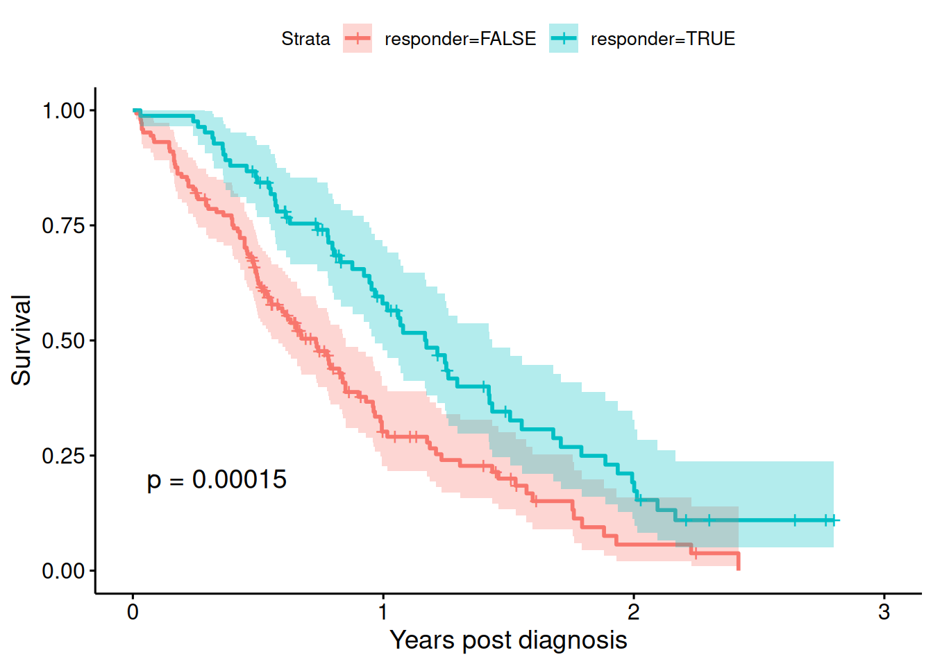
Figure 9.13: Kaplan-Meier estimate of the survival curves of patients with advanced lung cancer, by responder status (wrong analysis).
| Hazard Ratio | 95%-confidence interval | \(p\)-value |
|---|---|---|
| 0.54 | from 0.39 to 0.74 | 0.0002 |
There appears to be an effect of tumor response on survival, but it should not have an effect as responders were generated randomly. The analysis is flawed as it violates “Breslow’s first rule” and is subject to time-dependent bias. More precisely, the bias is that the probability to be a responder increases with time.
At the beginning, we do not know who becomes a responder. We should therefore treat it as a time-dependent covariate. For the correct analysis with time-dependent covariate, we need to split the data by responder status. This augmented data set looks as follows:
##   id tstart  tstop response status time endpt
## 1  1    0.0  306.0        0      2  306     2
## 2  2    0.0  152.5        0      2  455     0
## 3  2  152.5  455.0        1      2  455     2
## 4  3    0.0  183.0        0      1 1010     0
## 5  3  183.0 1010.0        1      1 1010     1
## 6 4 0.0 91.5 0 2 210 0| Hazard Ratio | 95%-confidence interval | \(p\)-value |
|---|---|---|
| 0.87 | from 0.61 to 1.23 | 0.42 |
In the correct analysis, there is no evidence for an effect of tumor response on survival, as it should be for randomly generated responders.
9.5 Additional references
Additional references are Bland (2015) (Ch. 16 Time to Event Data), Matthews (2006) (Sec. 7.5 Survival Analysis) and Collett (2003). The Pike hazard ratio estimate based on the output from the log-rank test is described in Berry et al (1991). Studies where the methods from this chapter are applied in practice are for example Blue et al (2001), Colorectal Cancer Collaborative Group (2000), Zar et al (2007).