Chapter 3 Clinical measurement and agreement

This chapter explores the potential bias and precision of clinical measurements, addressing both repeated measurements taken by the same observer and those taken by different observers. It introduces key concepts such as reliability, repeatability, and agreement.

3.1 Precision of clinical measurements

Significant figures inform about the precision with which measurements are being reported. They consist of all non-zero digits, zeros between non-zero digits, and zeros following the last non-zero after the decimal point. Significant figures are not the same as decimal places, which are all the digits after the decimal point. The difference between the two concepts is illustrated in Table 3.1. Observations should be rounded to a few significant figures only for reporting, after all the calculations have been done.

Table 3.1: Precision of reported measurements depends on the number of significant figures.
Reported measurement	Number of significant figures	Number of decimal places
1.5	2	1
0.15	2	2
1.66	3	2
0.0011	2	4
0.00110	3	5

3.1.1 Measurement error

Multiple measurements of the same quantity on the same subject will typically differ due to measurement error. To estimate the size of measurement error, the within-subject standard deviation, $s_w$ , can be calculated. To do so, a set of replicate readings is needed, where each subject in the sample is measured more than once. The within-subject standard deviation, $s_w$ , can then be calculated using one-way analysis of variance (ANOVA).

Example 3.1 A peak flow meter is a device to measure the maximal expiration speed of a person (faster = “better”). The Peak Expiratory Flow Rate (PEFR) data from Bland (2015) (Chapter 20.2) contains 17 pairs of readings made by the same observer with a Wright Peak Flow Meter (in litres/min) on 17 healthy volunteers, see Figure 3.1.

head(PEFR, 12)

##    Subject First Second
## 1        1   494    490
## 2        2   395    397
## 3        3   516    512
## 4        4   434    401
## 5        5   476    470
## 6        6   557    611
## 7        7   413    415
## 8        8   442    431
## 9        9   650    638
## 10      10   433    429
## 11      11   417    420
## 12      12   656    633

Figure 3.1: Repeated measurements of peak expiratory flow rate (Bland, 2015)

Example 3.2 The TONE study is a randomized controlled trial aimed at determining whether a reduction in sodium intake can effectively control blood pressure (Appel et al, 1995). Nab et al (2021) simulated a dataset based on the TONE study, containing for each participant: the sodium intake in mg measured by a 24h recall, a binary variable indicating whether the participant was assigned to a usual or sodium-lowering diet, and two measurements of sodium intake in mg measured in urine. We focus here on the participants for which the two urinary measurements are available. The two sodium intake measurements are displayed in Figure 3.2.

Repeated measurements of urinary sodium intake [@Nab2021].

Figure 3.2: Repeated measurements of urinary sodium intake (Nab et al, 2021).

The one-way ANOVA for the PEFR date (Example 3.1) is computed as follows:

measurement <- c(First, Second)
print(n <- nrow(PEFR))

## [1] 17

subject <- as.factor(rep(Subject, 2))

my.aov <- aov(measurement ~ subject)
summary(my.aov)

##             Df Sum Sq Mean Sq F value   Pr(>F)    
## subject     16 441599   27600   117.8 3.15e-14 ***
## Residuals   17   3983     234                     
## ---
## Signif. codes:  
## 0 '***' 0.001 '**' 0.01 '*' 0.05 '.' 0.1 ' ' 1

The entry Residuals Mean Sq gives the within-subject variance $s_w^2 = 234$ , so the within-subject standard deviation is $s_w = \sqrt{234} = {15.3}$ litres/min.

For the sodium data (Example 3.2), the within-subject standard deviation is calculated with the following Rcode:

measurement_sod <- c(sodium_f$urinary1, sodium_f$urinary2)
subject_sod <- rep(1:nrow(sodium_f), times = 2)

aov_sod <- aov(measurement_sod ~ subject_sod)
(sigmaw_sod <- sqrt(summary(aov_sod)[[1]][2,3]))

## [1] 0.6128869

and so $s_w = 0.6$ mg.

It is also possible to calculate a confidence interval for the within-subject standard deviation $s_w$ using the following R function:

confintSD <- function(sd, dof, level = 0.95){
  alpha <- 1 - level
  p_lower <- alpha/2
  p_upper <- 1-alpha/2
  c(lower = sqrt(dof / qchisq(p_upper, df = dof)) * sd,
    estimate = sd, 
    upper = sqrt(dof / qchisq(p_lower, df = dof)) * sd)
}

# for PEFR data
round(confintSD(sd = sigmaw, dof = 17), 1)

##    lower estimate    upper 
##     11.5     15.3     22.9

# for sodium data
round(confintSD(sd = sigmaw_sod, dof = nrow(sodium_f)), 2)

##    lower estimate    upper 
##     0.58     0.61     0.65

Derivation details are given in Appendix A.5.

A simpler way to compute $s^2_w$ (which gives approximately the same result) is based on the variance $s^2_d$ of the differences Diff between the two measurements, $s^2_w = s^2_d/2$ . For the PEFR data (Example 3.1), this gives

## compute the differences
PEFR$Diff <- PEFR[, "First"]-PEFR[, "Second"]

## variance of the differences
varDiff <- var(PEFR$Diff)

## within-subject variance is half the variance of the differences
varWithin <- varDiff/2
sw <- sqrt(varWithin)
print(round(sw, 1))

## [1] 15.4

However, this approach cannot be used if there are more than two measurements for some subjects.

3.1.2 Measurement error related to size

Sometimes measurement error is proportional to the size of the measurement. If this is the case, a logarithmic transformation of the measurements may be helpful. If there are two measurements per subject, the (rank) correlation between the absolute value of the difference between two measurements and the mean of the two measurements can be used to check whether such a transformation is needed, see Figure 3.3 for the PEFR and the sodium data (Examples 3.1 and 3.2, respectively).

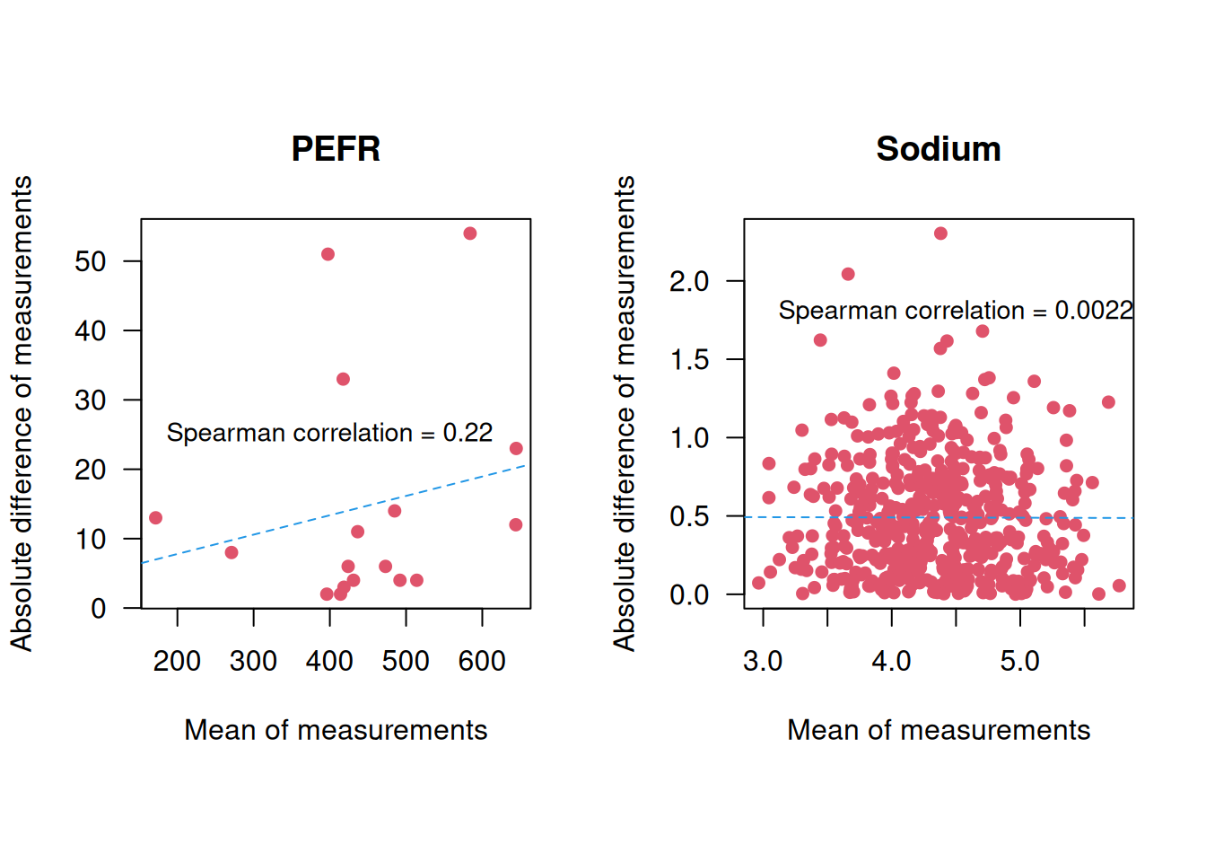
Figure 3.3: Absolute difference against mean of the two measurements.

(ctest_pefr <- cor.test(x_pefr, y_pefr, method="spearman"))

## 
##  Spearman's rank correlation rho
## 
## data:  x_pefr and y_pefr
## S = 640.35, p-value = 0.4067
## alternative hypothesis: true rho is not equal to 0
## sample estimates:
##       rho 
## 0.2152536

(ctest_sod <- cor.test(x_sod, y_sod, method="spearman"))

## 
##  Spearman's rank correlation rho
## 
## data:  x_sod and y_sod
## S = 20538650, p-value = 0.9607
## alternative hypothesis: true rho is not equal to 0
## sample estimates:
##         rho 
## 0.002215237

Spearman’s rank correlation coefficient in the PEFR example ( $\rho_S = 0.22$ ) is larger than in the sodium example ( $\rho_S = 0.0022$ ), but the $P$ -value for the correlation test is large in both cases ( $p=0.41$ and $p=0.96$ , respectively). Hence there is no evidence for an association between the mean measurement and the absolute difference of the measurements, so no transformation is required.

Example 3.3 Bland and Altman (1996) report the duplicate salivary cotinine measurements for a group of 20 Scottish schoolchildren, see Figure 3.4.

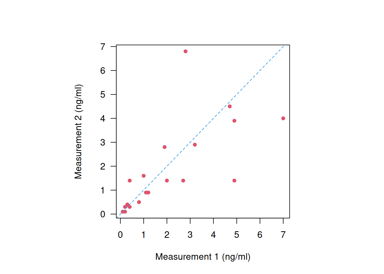
$Measurement 1 versus Measurement 2 for the 20 schoolchildren in Example \@ref(exm:cotinine).$

Figure 3.4: Measurement 1 versus Measurement 2 for the 20 schoolchildren in Example 3.3.

There is a strong correlation between the absolute value of the difference of the two measurements and the mean of the two measurements ( $\rho_S$ = 0.84, $p$ < 0.0001). This correlation becomes small when log measurements are used ( $\rho_S$ = 0.06, $p$ = 0.80), see Figure 3.5.

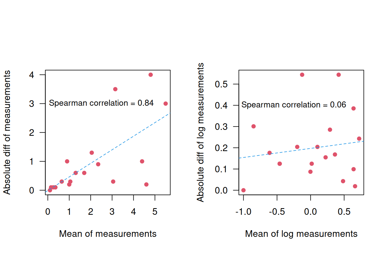
$Absolute difference versus mean of measurement (left) or log measurements (right) for the Example \@ref(exm:cotinine).$

Figure 3.5: Absolute difference versus mean of measurement (left) or log measurements (right) for the Example 3.3.

3.1.3 Repeatability

Definition 3.1 Repeatability is the value below which the difference $d$ between two measurements will lie with a certain probability, usually 0.95.

Repeatability is usually computed as $1.96 \sqrt{2} s_w \approx 2 \sqrt{2} s_w \approx 2.8 s_w$ , where $s_w$ is the within-subjects standard deviation. Note that the standard deviation of $d$ is $s_d = \sqrt{2} s_w$ . The repeatability is $43.3$ litres/min in the PERF data (Example 3.1) with 95% CI

##    lower estimate    upper 
##     32.5     43.3     64.9

and $1.7$ mg in the sodium data (Example 3.2) with 95% CI

##    lower estimate    upper 
##      1.3      1.7      2.6

The limits of the confidence interval for $2\sqrt{2}s_w$ are calculated by multiplying the limits of the confidence interval for $s_w$ by $2\sqrt{2}$ .

The value $2 \sqrt{2} s_w$ is also called the smallest real difference, because it is the smallest difference that can be interpreted as evidence for a real change in the subject’s true value.

3.1.4 Reliability and the intraclass correlation coefficient

Definition 3.2 Reliability refers to the correlation between pairs of readings.

Pearson correlation coefficient between the first and second measurement depends on the ordering of pairs and is therefore not appropriate to assess the reliability between two pairs of measurements. To illustrate this problem we change the ordering of some random pairs in the PERF data:

print(switch.me)

## [1]  1  2  4  7 11 13 14 16

print(head(cbind(First, Second, First.new, Second.new)))

##      First Second First.new Second.new
## [1,]   494    490       490        494
## [2,]   395    397       397        395
## [3,]   516    512       516        512
## [4,]   434    401       401        434
## [5,]   476    470       476        470
## [6,]   557    611       557        611

cor(First, Second)

## [1] 0.9834307

## cor(First.new, Second.new) not the same as cor(First, Second)
cor(First.new, Second.new)

## [1] 0.9823037

In contrast, the intraclass correlation coefficient (ICC) does not depend on the ordering of the pairs and should be used instead. The ICC is the average correlation among all possible ordering of pairs and extends easily to the case of more than two observations per subject. It can be defined based on the between- and within-subject variances:

Definition 3.3 The Intraclass Correlation Coefficient (ICC) relates the between-subject variance $s_b^2$ to the total variance $s_b^2 + s_w^2$ of the measurements: $\begin{equation*} \mathrm{ICC} = \frac{s_b^2}{s_b^2 + s_w^2}. \end{equation*}$

The between-subject variance $s^2_b$ can also be read-off from an ANOVA, $s^2_b =$ (subject Mean Sq $-$ Residuals Mean Sq) $/2$ .

A convenient way to compute ICC is to use the function ICC::ICCbare():

library(ICC) 
ICCbare(x=as.factor(subject), y=measurement)

## [1] 0.983165

The ICC package also provides a function to calculate confidence intervals for the ICC:

sel <- c("LowerCI", "ICC", "UpperCI")
## Compute CIs
ICC.CI <- ICCest(x=subject, y=measurement)[sel]

print(t(ICC.CI))

##      LowerCI   ICC      UpperCI  
## [1,] 0.9552393 0.983165 0.9938183

ICC can be interpreted as the proportion of the variance of measurements which is due to the variation between true values rather than to measurement error. Therefore ICC depends on the variation between subjects and thus relates to the population from which the sample was taken. This method should hence be used only when we have a representative sample of the subjects of interest (Bland, 2015).

Example 3.1 (continued) For illustration we modify the PERF data to have less variation between subjects, but the same within-subject standard deviation, see Figure 3.6.

mymeans <- apply(cbind(First, Second), 1, mean)
shrinkage <-  0.5*(mymeans-mean(mymeans))
ShrunkenFirst <- First - shrinkage
ShrunkenSecond <- Second - shrinkage
ShrunkenMeasurement <- c(ShrunkenFirst, ShrunkenSecond)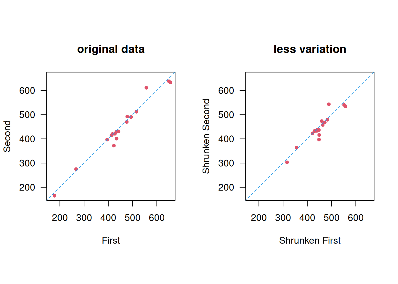

Figure 3.6: Less between-subject variation.

my.aov <- aov(ShrunkenMeasurement ~ subject)
summary(my.aov)

##             Df Sum Sq Mean Sq F value   Pr(>F)    
## subject     16 110400    6900   29.45 2.79e-09 ***
## Residuals   17   3983     234                     
## ---
## Signif. codes:  
## 0 '***' 0.001 '**' 0.01 '*' 0.05 '.' 0.1 ' ' 1

The within-subject standard deviation doesn’t change: $s_w = \sqrt{234} = {15.3}$ litres/min, but the ICC is smaller:

ICCbare(x=as.factor(subject), y=ShrunkenMeasurement)

## [1] 0.9343187

3.2 Agreement of two methods with continuous measurements

In Section 3.1, we discussed repeatability and reliability, focusing on how well replicates from the same observer align. Now, the focus shifts to examining the agreement between different observers (subjects, machines, methods, etc.).

Example 3.4 A total of $n=39$ pairs of blood glucose measurements (in mmol/L) were measured with two different devices: the Cobas6000 and the Hitachi912. Figure 3.7 displays the results from a correlation and a regression analysis to assess the agreement between the two devices. However, neither of these methods is useful to assess agreement.

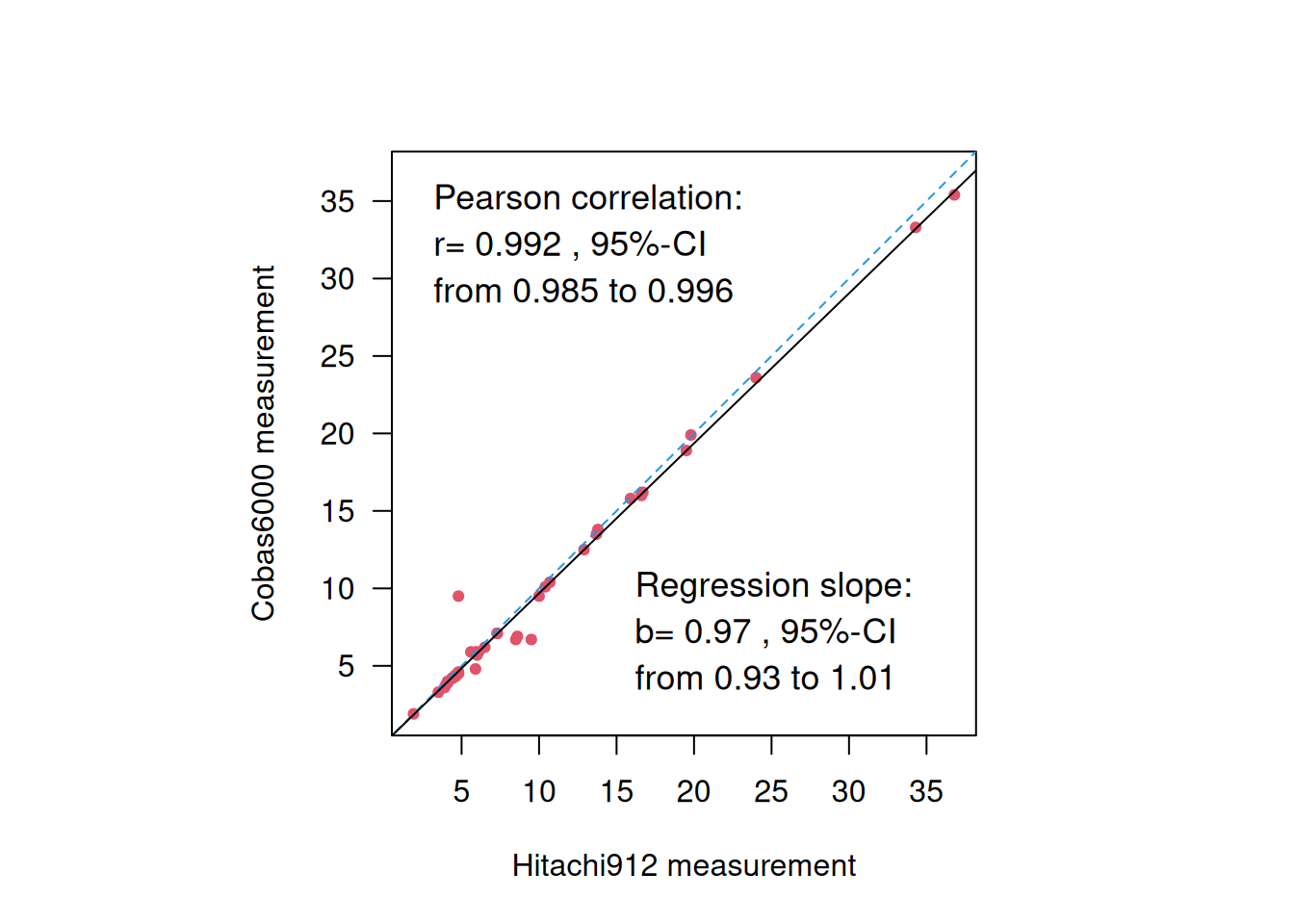
Figure 3.7: Blood glucose measurements from two different devices.

First, correlation is not useful to assess agreement, because multiplication of measurements from one device with any factor will not change the correlation, so devices that do not agree may show high correlation. For example, the correlation between 10 $\times$ Cobas6000 and Hitachi912 measurements remains the same:

(cor.test(10*co, hi))

## 
##  Pearson's product-moment correlation
## 
## data:  10 * co and hi
## t = 48.211, df = 37, p-value < 2.2e-16
## alternative hypothesis: true correlation is not equal to 0
## 95 percent confidence interval:
##  0.9849374 0.9958996
## sample estimates:
##       cor 
## 0.9921343

Furthermore, a regression slope $b \approx 1$ does also not necessarily mean good agreement, because adding a constant to the measurements from one device will not change the regression slope, so two methods that do not agree may still have a slope $\approx$ 1. For example the regression slope for 10 + Cobas6000 vs. Hitachi912 measurements remains around 1:

knitr::kable(biostatUZH::tableRegression(lm(10 + co ~ hi),
                                         xtable = F))

	Coefficient	95%-confidence interval	$p$ -value
Intercept	10.00	from 9.48 to 10.52	< 0.0001
hi	0.97	from 0.93 to 1.01	< 0.0001

3.3 The method of Bland & Altman

The method of Bland & Altman was introduced in 1986, see the original publication in Figure 3.8. It extends the concept of repeatability introduced in Section 3.1.3 to observations from different devices to introduce the limits of agreement. The original publication is one of the most cited papers in medical research with more than 50’000 citations by the end of 2023.

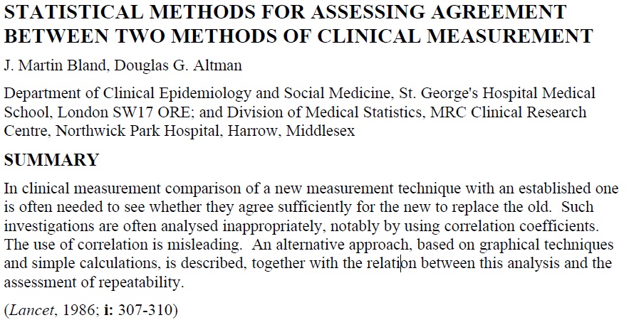
Figure 3.8: The original publication by Bland & Altman.

The Bland-Altman plot assesses the dependency of measurement error (size and variability) on the “true” value. The $x$ -axis gives the mean $(x_i + y_i)/2$ of both measurements as an estimate of true value. The $y$ -axis gives the difference $d_i = x_i - y_i$ of both measurements to eliminate variability between observations. The bias, i.e. the mean difference $\bar{d}$ (systematic error) with its confidence interval, and the limits of agreement (LoA) can be read off the Bland-Altman plot. Approximately 95% of points will lie between

$\underbrace{\bar{d} - 2 \cdot s_d}_{\mbox{LoA}_{\tiny \mbox{low}}} \mbox{ and } \underbrace{\bar{d} + 2 \cdot s_d}_{\mbox{LoA}_{\tiny \mbox{up}}}.$

Here $s_d=\sqrt{2} s_w$ is the standard deviation of the differences. If differences within the limits of agreement are considered not clinically relevant then the two methods are considered exchangeable.

3.3.1 Confidence intervals for limits of agreement

Under normality, $\bar{d}$ and $s_d$ are independent. The variance of $\bar d$ is estimated by $s_d^2/n$ , with $n$ the sample size. The variance of $s_d$ can be approximately estimated by $s_d^2/2n$ [see Bland and Altman (1986); Bland and Altman (1999); Appendix A.5]. Hence, the standard error of the limits of agreement is estimated by $\begin{eqnarray*} \mbox{se}(\mbox{LoA}_{\tiny \mbox{low}}) = &\mbox{se}(\mbox{LoA}_{\tiny \mbox{up}}) \\ = & \mbox{se}(\bar{d} \pm 2 \cdot s_d) \\ = & \sqrt{\mathop{\mathrm{Var}}(\bar{d} \pm 2 \cdot s_d)} \\ = & \sqrt{\mathop{\mathrm{Var}}(\bar d) + 4 \mathop{\mathrm{Var}}(s_d)} \\ \approx & \sqrt{s_d^2/n + 4 s_d^2/2n} \\ = & \sqrt{3/n} \, s_d \ . \end{eqnarray*}$ This can be used to compute 95% CI for $\mbox{LoA}_{\tiny \mbox{low}}$ and $\mbox{LoA}_{\tiny \mbox{up}}$ . The standard error can also be used to compute the required sample size $n$ for a fixed width $w$ of the 95% confidence interval for the limits of agreement. A rule of thumb by Martin Bland is: “I usually recommend $n$ =100 as a good sample size, which gives a 95% CI about $\pm$ 0.34 $s_d$ .”

Example 3.4 (continued) The Bland-Altman plot for the glucose measurements is shown in Figure 3.9. The bias is 0.32 mmol/L with 95% CI from -0.01 to 0.65 (left). The limits of agreement are $\mbox{LoA}_{\tiny \mbox{low}}$ = -1.67 mmol/L with 95% CI from -2.24 to -1.10 and $\mbox{LoA}_{\tiny \mbox{up}}$ = 2.30 mmol/L with 95% CI from 1.74 to 2.87 (right).

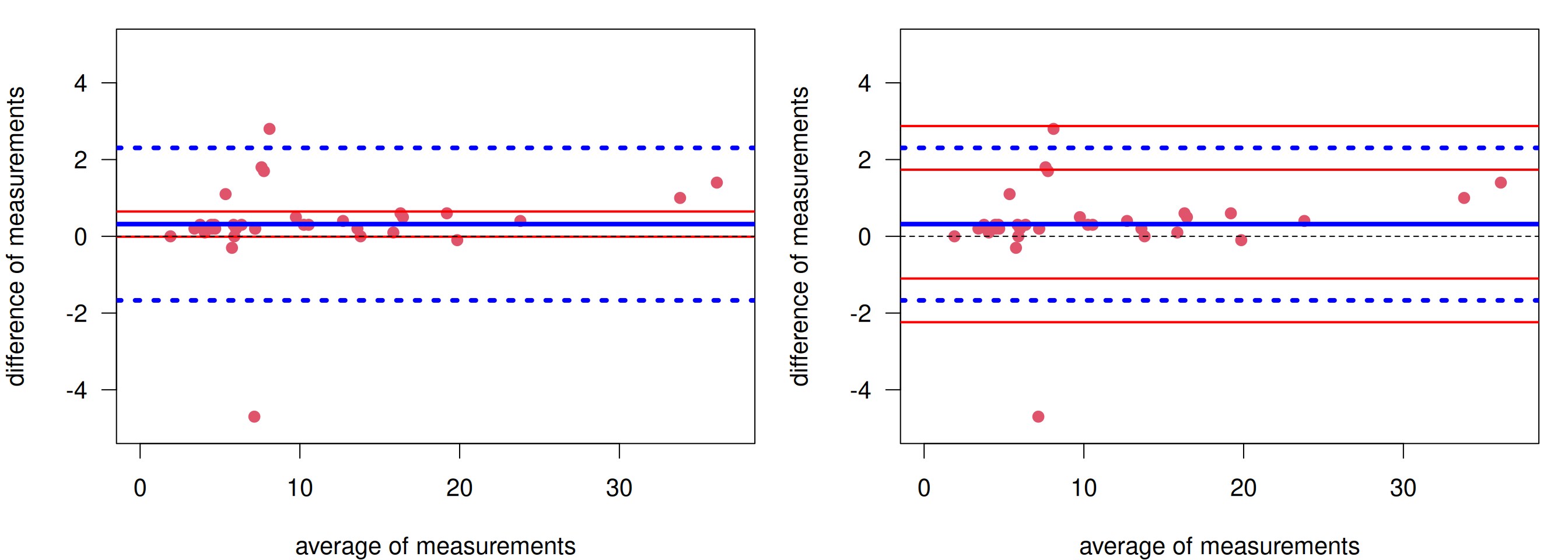
Bland-Altman plot for glucose measurements. Left: With confidence interval for the bias. Right: With confidence intervals for the limits of agreement.

Figure 3.9: Bland-Altman plot for glucose measurements. Left: With confidence interval for the bias. Right: With confidence intervals for the limits of agreement.

In order to know whether Hitachi912 can be replaced with Cobas6000, one has to determine a priori what difference $\delta$ is clinically relevant. If the limits of agreement (lower = -1.67, upper = 2.30) (or the corresponding confidence intervals) are within $[-\delta, \delta]$ , then the old device can be replaced.

3.4 Agreement of two methods with binary variables

Example 3.5 179 patients completed a Symptom Interpretation Questionnaire on two occasions three years apart. Each time, they were were classified into “normalizer” and “non-normalizer”, related to how they were able to cope with symptoms (Kirkwood and Sterne, 2003, pp. 434, Ex.36.3).

Table 3.2: Agreement of binary classification of patients on two occasions three years apart.
	Second classification
First classification	Normalizer	Non-normalizer	Total
Normalizer	76	17	93
Non-normalizer	39	47	86
Total	115	64	179

The proportion of agreement between the two classifications is $\begin{eqnarray*} p_\mathrm{obs}&=& (76 + 47) / 179 \ = \ 0.69. \end{eqnarray*}$ The problem is that two “random” classifiers would also agree for some patients, so we need to adjust for this agreement by chance. We can calculate this based on the expected frequencies under independence. For example, the expected frequency in the first cell of Table 3.2 is $115 \cdot 93 / 179 = 59.7$ .

Table 3.3: Table of expected frequencies of agreement by chance, given row- and column totals.
	Second classification
First classification	Normalizer	Non-normalizer	Total
Normalizer	59.7	33.3	93
Non-normalizer	55.3	30.7	86
Total	115.0	64.0	179

Table 3.3 gives all four expected frequencies. The expected proportion of agreement by chance then is $\begin{eqnarray*} p_\mathrm{exp}%&=& (n_{1+} n_{+1} + n_{2 +} n_{+ 2})/n_{++}^2 \\ &=& (59.7 + 30.7) / 179 \\ &=& 0.51. \end{eqnarray*}$

3.4.1 Cohen’s Kappa

Definition 3.4 Cohen’s Kappa is the proportion of agreement beyond chance $p_\mathrm{obs}- p_\mathrm{exp}$ , standardized with the maximal possible value $1-p_\mathrm{exp}$ :

$\begin{eqnarray*} \kappa &=& \frac{p_\mathrm{obs}- p_\mathrm{exp}}{1 - p_\mathrm{exp}} \end{eqnarray*}$

It has the following properties: $\kappa \leq p_\mathrm{obs}$ , $\kappa = 1$ means that there is perfect agreement ( $p_\mathrm{obs}=1$ ), $\kappa = 0$ mean that the agreement not larger than expected by chace ( $p_\mathrm{obs}=p_\mathrm{exp}$ ), and the smallest possible value of $\kappa$ is $-p_\mathrm{exp}/(1-p_\mathrm{exp})$ .

In Example 3.5 we obtain

$\begin{eqnarray*} \kappa &=& \frac{0.69- 0.51}{1 - 0.51} = 0.37. \end{eqnarray*}$

A classification of Cohen’s Kappa from Altman (1991) and Bland (2015) is given in Table 3.4.

Table 3.4: Classification of Cohen’s Kappa Bland (2015).
Value of kappa	Strength of agreement
$0.00 - 0.20$	Poor
$0.21 - 0.40$	Fair
$0.41 - 0.60$	Moderate
$0.61 - 0.80$	Good
$0.81 - 1.00$	Very good

However, there is a caveat with the interpretation shown in Table 3.4: $\kappa$ also depends on the true proportion of subjects in the two categories. Figure 3.10 shows the expected $\kappa$ as a function of the true proportion of “Yes” subjects for different probabilities of agreement. We can see that expected $\kappa$ drops for extreme proportions close to zero or one.

In Table 3.5, $\kappa = 0.37$ although $p_\mathrm{obs}= 123$ / $179$ = $0.69$ . The problem is that the observed proportion of “positive” subjects is very low (5/94 resp. 6/94). This shows that $\kappa$ also depends on the marginal distribution of positive (respectively negative) subjects!

$Dependence of $\kappa$ on the true proportion of positive subjects.$

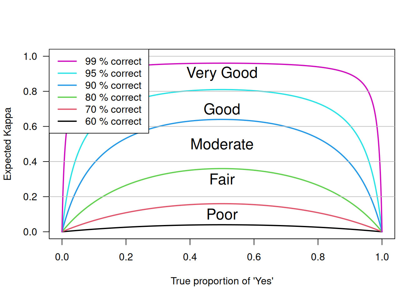
Figure 3.10: Dependence of $\kappa$ on the true proportion of positive subjects.

Table 3.5: Extreme example for interpretation of Kappa.
	Rater 2
Rater 1	negative	positive	Total
negative	84	4	88
positive	5	1	6
Total	89	5	94

3.4.2 Confidence Interval for Cohen’s Kappa

The standard error of $\kappa$ is

$\mbox{se}( \kappa) %% = \frac{\SE(\pobs)}{1-\pexp} = \frac{\sqrt{p_\mathrm{obs}\, (1- p_\mathrm{obs})}} {(1- p_\mathrm{exp}) \sqrt{n}},$

so a Wald confidence interval for $\kappa$ can be easily computed. Using the substitution method, a Wilson interval for $p_\mathrm{obs}$ can be used to obtain a confidence interval for $\kappa$ with better properties. For small $n$ , bootstrap CIs might be even better, which would also incorporate uncertainty with respect to $p_\mathrm{exp}$ .

The different confidence intervals require different formats of the data: The Wald CI requires data in aggregated form (the ordinary $2 \times 2$ table format):

print(symptoms)

##                    **Normalizer** **Non-normalizer**
## **Normalizer**                 76                 17
## **Non-normalizer**             39                 47

In contrast, the bootstrap CI needs data on individual level, with each row representing the measurements from one subject:

print(head(symptoms.ind))

##   First Second
## 1     1      1
## 2     1      1
## 3     1      1
## 4     1      1
## 5     1      1
## 6     1      1

A Wald confidence interval is obtained conveniently using psych::cohen.kappa():

library(psych)
cohen.kappa(symptoms)

## Call: cohen.kappa1(x = x, w = w, n.obs = n.obs, alpha = alpha, levels = levels)
## 
## Cohen Kappa and Weighted Kappa correlation coefficients and confidence boundaries 
##                  lower estimate upper
## unweighted kappa  0.23     0.37   0.5
## weighted kappa    0.23     0.37   0.5
## 
##  Number of subjects = 179

The Wilson confidence interval requires transformation of the confidence limits of $p_\mathrm{obs}$ to $\kappa$ :

pobsCI <- wilson(x=sum(diag(symptoms)), n=sum(symptoms))
pexp <- sum(diag(chisq.test(symptoms)$expected)/sum(symptoms))
round((pobsCI-pexp)/(1-pexp), 2)

## lower  prop upper 
##  0.22  0.37  0.50

A 95% bootstrap CI for Cohen’s Kappa is obtained using biostatUZH::confIntKappa():

res <- biostatUZH::confIntKappa(symptoms.ind, type="Cohen")

## Caution, used levels in weighted Kappa: 0, 1

round(res$boot.quant, 2)

##  2.5% 97.5% 
##  0.22  0.49

3.4.3 Weighted Kappa

It might happen that more than two categories are of interest.

Example 3.6 The physical health of 366 subjects has been judged by a health visitor (HV) and the subject’s general practitioners (GP) (Bland, 2015). Table 3.6 shows the data (columns: HV, rows: GP).

Table 3.6: Data from Example 3.6.
	Poor	Fair	Good	Excellent
Poor	2	12	8	0
Fair	9	35	43	7
Good	4	36	103	40
Excellent	1	8	36	22

As a start we may only consider the diagonal entries for the assessment of agreement. This is unweighted kappa, calculated with $\begin{eqnarray*} p_\mathrm{obs}= \sum_{i=1}^{k} p_{ii}, \\ p_\mathrm{exp}= \sum_{i = 1}^k p_{i\cdot} p_{\cdot i} \end{eqnarray*}$ where $k$ is the number of categories, $p_{ij}$ is the observed relative frequency in cell ( $i$ , $j$ ), while $p_{i\cdot}$ and $p_{\cdot i}$ are the corresponding row and column sums.

However, agreement for ordinal variables is better based on the weighted $\kappa_w$ with weights of agreement $w_{ij}$ :

$\begin{eqnarray*} p_\mathrm{obs}&=& \sum_{i=1}^{k}\sum_{j=1}^{k} w_{ij}p_{ij}, \\ p_\mathrm{exp}&=& \sum_{i = 1}^k\sum_{j=1}^{k} w_{ij}p_{i \cdot} p_{\cdot j}, \\ \kappa_w &=& \frac{p_\mathrm{obs}-p_\mathrm{exp}}{1-p_\mathrm{exp}}. \end{eqnarray*}$ The standard error of $\kappa_w$ is also available.

Common choices for the weight are quadratic and linear weights.

Quadratic weights:

##           Poor Fair Good Excellent
## Poor      1.00 0.89 0.56      0.00
## Fair      0.89 1.00 0.89      0.56
## Good      0.56 0.89 1.00      0.89
## Excellent 0.00 0.56 0.89      1.00

Linear weights:

##           Poor Fair Good Excellent
## Poor      1.00 0.67 0.33      0.00
## Fair      0.67 1.00 0.67      0.33
## Good      0.33 0.67 1.00      0.67
## Excellent 0.00 0.33 0.67      1.00

Example 3.6 (continued) Analysing agreement of the health assessments from Table 3.6 with the unweighted and weighted $\kappa$ :

cohen.kappa(health)

## Call: cohen.kappa1(x = x, w = w, n.obs = n.obs, alpha = alpha, levels = levels)
## 
## Cohen Kappa and Weighted Kappa correlation coefficients and confidence boundaries 
##                  lower estimate upper
## unweighted kappa 0.053     0.13  0.20
## weighted kappa   0.266     0.35  0.44
## 
##  Number of subjects = 366

The function cohen.kappa() uses quadratic weights as default. The weighted $\kappa_w$ turns out to be larger than the unweighted $\kappa$ .

3.5 Additional references

Literature on this topic includes Chapter 13 in Altman et al (2000) and Chapter 20 on clinical measurements in Bland (2015). Methodological discussions can be found in the Statistics Notes Altman and Bland (1996a), Altman and Bland (1996b), and Altman and Bland (1996c). Studies where the methods from this chapter are used in practice are for example Islami et al (2009), Little et al (2002), and Spector et al (1995).

References

Altman, D G 1991 Practical Statistics for Medical Research. London: Chapman & Hall.

Altman, D G and Bland, M J 1996a Statistics Notes: Measurement error. BMJ, 313: 744. DOI: https://doi.org/10.1136/bmj.313.7059.744

Altman, D G and Bland, M J 1996b Statistics Notes: Measurement error and correlation coefficients. BMJ, 313: 41–42. DOI: https://doi.org/10.1136/bmj.313.7048.41

Altman, D G and Bland, M J 1996c Statistics Notes: Measurement error proportional to the mean. BMJ, 313: 106. DOI: https://doi.org/10.1136/bmj.313.7049.106

Altman, D G, Machin, D, Bryant, T N, and Gardner, M J 2000 Statistics with Confidence. Second Edition. BMJ Books.

Appel, L J, Espeland, M, Whelton, P K, Dolecek, T, Kumanyika, S, Applegate, W B, Ettinger, W H, Kostis, J B, Wilson, A C, Lacy, C, and Miller, S T 1995 Trial of nonpharmacologic intervention in the elderly (TONE). Annals of Epidemiology, 5(2): 119–129. DOI: https://doi.org/10.1016/1047-2797(94)00056-y

Bland, M J 2015 An Introduction to Medical Statistics. Fourth Edition. Oxford University Press.

Bland, M J and Altman, D G 1999 Measuring agreement in method comparison studies. Statistical Methods in Medical Research, 8(2): 135–160. DOI: https://doi.org/10.1177/096228029900800204

Bland, M J and Altman, D G 1996 Statistics notes: Measurement error proportional to the mean. BMJ, 313(7049): 106–106. DOI: https://doi.org/10.1136/bmj.313.7049.106

Bland, M J and Altman, D G 1986 Statistical methods for assessing the agreement between two methods of clinical measurements. Lancet, 1: 307–310. DOI: https://doi.org/10.1016/S0140-6736(86)90837-8

Islami, F, Pourshams, A, Nasrollahzadeh, D, Kamangar, F, Fahimi, S, Shakeri, R, Abedi-Ardekani, B, Merat, S, Vahedi, H, Semnani, S, Abnet, C C, Brennan, P, Møller, H, Saidi, F, Dawsey, S M, Malekzadeh, R, and Boffetta, P 2009 Tea drinking habits and oesophageal cancer in a high risk area in northern Iran: population based case-control study. BMJ, 338: 1–6. DOI: https://doi.org/10.1136/bmj.b929

Kirkwood, B R and Sterne, J A C 2003 Essential Medical Statistics. Second Edition. Blackwell Publishing.

Little, P, Barnett, J, Barnsley, L, Marjoram, J, Fitzgerald-Barron, A, and Mant, D 2002 Comparison of agreement between different measures of blood pressure in primary care and daytime ambulatory blood pressure. BMJ, 325: 1–6. DOI: https://doi.org/10.1136/bmj.325.7358.254

Nab, L, Smeden, M van, Keogh, R H, and Groenwold, R H H 2021 Mecor: An r package for measurement error correction in linear regression models with a continuous outcome. Computer Methods and Programs in Biomedicine, 208: 106238. DOI: https://doi.org/10.1016/j.cmpb.2021.106238

Spector, T D, Keen, R W, Arden, N K, Morrison, N A, Major, P J, Nguyen, T V, Kelly, P J, Baker, J R, Sambrook, P N, Lanchbury, J S, and Eisman, J A 1995 Influence of vitamin D receptor genotype on bone mineral density in postmenopausal women: a twin study in Britain. BMJ, 310: 1357–1360. DOI: https://doi.org/10.1136/bmj.310.6991.1357