Chapter 1 Binary diagnostic tests
1.1 Diagnostic accuracy studies
A binary diagnostic test categorizes individuals as either diseased or non-diseased. Examples of diagnostic tests include mammography for the diagnosis of breast cancer, pap smear screening for the diagnosis of cervical cancer, and prostate-specific antigen (PSA) screening for the diagnosis of prostate cancer. Continuous diagnostic tests (such as the actual PSA measurements) are often dichotomized to binary tests using a suitable threshold, see Chapter 2.
1.1.1 Study designs
The study design determines the selection of study subjects from a population. In a case-control design, a diagnostic test is applied to a sample of diseased and non-diseased individuals, with a fixed sample size for both groups. In a cohort design, a diagnostic test is applied to a sample of subjects from the population of interest, and the true disease status is also ascertained using a reference test, the gold standard.
Moreover, studies comparing two tests can have an unpaired or a paired design. In an unpaired design, each study subject is tested with only one of the two tests. In contrast, each study subject is tested with both tests in a paired design.
1.1.2 Test integrity
Knowledge of the true disease status of the individual must not influence the assessment of the diagnostic test. For example, if a radiologist is aware that a woman has breast cancer, she/he may scrutinize her mammogram more closely for signs of cancer, introducing a potential bias. In order to address this issue, blinding should be used. This means that the person who applies the diagnostic test must not know the true disease status, and the person who determines the true disease status (using a reference/gold standard test) must not know the test result.
Example 1.1 The Million Women Study (MW Study) is a cohort study of women’s health analyzing data from more than one million women aged 50 and over (Oxford Population Health, 1996). 122’355 women between 50 and 64 years underwent a mammography and have been followed-up for a year to determine whether or not they have been diagnosed with breast cancer, confirmed via histology (the gold standard). The results are summarized in Table 1.1.
| Mammography | no | yes | Total |
|---|---|---|---|
| negative | 117,744 | 97 | 117,841 |
| positive | 3,885 | 629 | 4,514 |
| Total | 121,629 | 726 | 122,355 |
1.2 Measures of diagnostic accuracy
The following notation is used for binary diagnostic tests:
\[\begin{eqnarray*} D & = & \left\{ \begin{array}{ll} 1 & \mbox{diseased} \\ 0 & \mbox{non-diseased} \end{array} \right. \end{eqnarray*}\]
\[\begin{eqnarray*} Y & = & \left\{ \begin{array}{ll} 1 & \mbox{test positive for disease} \\ 0 & \mbox{test negative for disease} \end{array} \right. \end{eqnarray*}\]
Table 1.2 introduces our notation for the counts from a simple diagnostic accuracy study with total sample size \(n\). For the data from the MW study shown in Table 1.1 we have \(tp = 629\) true positives, \(fp = 3,885\) false positives, \(tn = 117,744\) true negatives, \(fn = 97\) false negatives, and a total sample size of \(n = 122,355\).
| \(D=0\) | \(D=1\) | Total | |
|---|---|---|---|
| \(Y=0\) | True negatives (\(tn\)) | False negatives (\(fn\)) | \(n^{-}\) |
| \(Y=1\) | False positives (\(fp\)) | True positives (\(tp\)) | \(n^{+}\) |
| Total | \(n_0\) | \(n_1\) | \(n\) |
1.2.1 Sensitivity and specificity
Definition 1.1 The sensitivity of a binary test is defined as
\[\begin{equation} \text{Sens} = \Pr(Y=1 \,\vert\,D=1), \end{equation}\]
that is, the probability of correctly identifying study subjects with a specific disease.
The specificity of a binary test is defined as
\[\begin{equation*} \text{Spec} = \Pr(Y=0 \,\vert\,D=0), \end{equation*}\]
that is, the probability of correctly identifying study subjects without a specific disease.
In the MW Study (Example 1.1), the following estimates for the sensitivity and specificity are obtained from Table 1.1:
\[\begin{eqnarray} \mbox{Sens} &=& \displaystyle\frac{{tp}}{{tp}+{fn}} = \displaystyle\frac{629}{726} = 86.6\% \mbox{ and} \\ \mbox{Spec} &=& \displaystyle\frac{{tn}}{{tn}+{fp}} = \displaystyle\frac{117,744}{121,629} = 96.8\% . \end{eqnarray}\]
Definition 1.2 Youden’s index is defined as
\[\begin{equation} J = \mbox{Sens} + \mbox{Spec} - 1 . \tag{1.1} \end{equation}\]
A categorization of test quality based on Youden’s index is shown in Table 1.3:
| Youden’s Index | Test quality |
|---|---|
| \(J=1\) | perfect |
| \(0<J<1\) | useful |
| \(J=0\) | useless |
| \(J<0\) | harmful |
A perfect test (\(J=1\)) must have both Sens \(=\) 1 and Spec \(=\) 1. A useless test (\(J=0\)) has Sens \(=\) 1 \(-\) Spec, so the probability of a positive test is the same for diseased and non-diseased individuals: \[\begin{eqnarray*} \mbox{Sens} & = & \Pr(Y=1 \,\vert\,D=1) \\ & = & 1 - \mbox{Spec} \\ & = & 1 - \Pr(Y=0 \,\vert\,D=0) \\ & = & \Pr(Y=1 \,\vert\,D=0). \end{eqnarray*}\]
A harmful test can be made useful by relabelling test results \(Y=1\) to \(Y=0\) and vice versa.
In the MW study (Example 1.1), we obtain \(J=0.866 + 0.968 - 1 = 0.83\), so mammography is a useful test to diagnose breast cancer according to Table 1.3.
Figure 1.1 illustrates that the same Youden’s index \(J\) can be achieved by very different combinations of sensitivity and specificity. For example, a diagnostic test with sensitivity 0.9 and specificity 0.7 will have the same Youden’s index \(J=0.6\) as a test with sensitivity 0.7 and specificity 0.9.
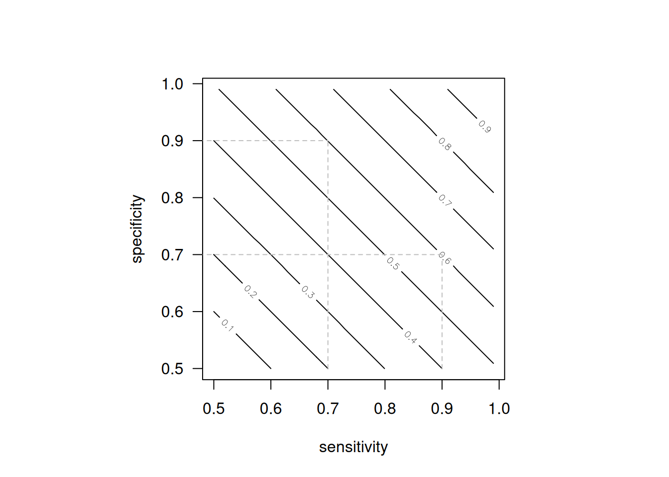
Figure 1.1: Contour plot of Youden’s index as a function of sensitivity and specificity.
1.2.2 Predictive values
The accuracy of a diagnostic test can also be described with predictive values.
Definition 1.3 The positive predictive value is defined as
\[\begin{equation*} \mbox{PPV} = \Pr(D=1 \,\vert\,Y=1), \end{equation*}\]
that is, the probability that a study subject with a positive test result actually has the disease.
The negative predictive value is defined as
\[\begin{equation*} \mbox{NPV} = \Pr(D=0 \,\vert\,Y=0), \end{equation*}\]
that is, the probability that a study subject with a negative test result actually does not have the disease.
Predictive values can be directly estimated in a cohort design (see Section 1.1.1), such as the MW study shown in Example 1.1:
\[\begin{eqnarray*} \mbox{PPV} &=& \displaystyle\frac{{tp}}{{tp}+{fp}} = 629/4,514 = 13.9\% \mbox{ and} \\ \mbox{NPV} &=& \displaystyle\frac{{tn}}{{tn}+{fn}} = 117,744/117,841 = 99.9\%. \end{eqnarray*}\] The negative predictive value NPV is close to 100%, which means that a woman with a negative mammogram is very likely not to have breast cancer. However, the positive predictive value is only 13.9%, so a woman with a positive mammogram still has a fairly small probability to have breast cancer.
This simple calculation assumes that the observed disease prevalence
\[\begin{eqnarray*} {\mbox{Prev}} = n_1/n = 726/122,355 &=& \, \, 0.6\% \end{eqnarray*}\]
in the study sample is representative for the underlying population.
Predictive values can also be calculated for other values of the prevalence with Bayes’ theorem:
\[\begin{eqnarray*} \mbox{PPV} & = & \frac{\mbox{Sens} \cdot \mbox{Prev}}{\mbox{Sens} \cdot \mbox{Prev} + (1-\mbox{Spec}) \cdot (1-\mbox{Prev})} \mbox{ and} \\ \mbox{NPV} & = & \frac{\mbox{Spec} \cdot (1-\mbox{Prev})}{\mbox{Spec} \cdot (1-\mbox{Prev}) + (1-\mbox{Sens}) \cdot \mbox{Prev}} \end{eqnarray*}\]
as the transition from pre-test probability of disease (the prevalence) to post-test probabilities of disease (\(\mbox{PPV}\) and \(\mbox{NPV}\)) after observing a positive, or negative test result. Table 1.4 gives predictive values in the MW study also for other values of the prevalence. As the prevalence increases, the PPV increases, while the NPV decreases.
Example 1.1 (continued) Cancer Research UK report a breast cancer prevalence of 4.5% for 59-year old British women. The corresponding predictive values are shown in the third row of Table 1.4: the positive predictive value is only 56% whereas the negative predictive value is 99%.
| Prevalence | PPV | NPV |
|---|---|---|
| 0.6% | 14% | 100% |
| 1.0% | 22% | 100% |
| 4.5% | 56% | 99% |
| 10.0% | 75% | 98% |
1.2.3 Likelihood ratios
Likelihood ratios are an alternative way for summarizing the accuracy of diagnostic tests.
Definition 1.4 The positive likelihood ratio is defined as
\[\begin{equation*} \mbox{LR}^+ = \frac{\mbox{Sens}}{1-\mbox{Spec}} \mbox{ and} \end{equation*}\]
the negative likelihood ratio as
\[\begin{equation*} \mbox{LR}^- = \frac{1-\mbox{Sens}}{\mbox{Spec}}. \end{equation*}\]
Likelihood ratios are ratios of probabilities and summarise how many times more (or less) likely study subjects with the disease are to have a particular test result (\(\mbox{LR}^+\) for a positive result, \(\mbox{LR}^-\) for a negative result) than study subjects without the disease. In contrast to predictive values, they do not depend on disease prevalence.
Useful tests have \(\mbox{LR}^+ > 1\) and \(\mbox{LR}^- < 1\). Likelihood ratios above 10 and below 0.1 are considered to provide strong evidence to rule in or rule out diagnoses (Deeks and Altman, 2004), respectively.
In the MW study (Example 1.1) we obtain: \[\begin{align*} \mbox{LR}^+ = \frac{86.6\%}{3.2\%} = {27.1} \ &\mbox{ and } \mbox{LR}^- = \frac{13.4\%}{96.8\%} = {0.14} \approx {1/7}. \end{align*}\]
1.2.4 Bayesian updating with likelihood ratios
LRs quantify the change in disease odds after having observed a positive or negative test result:
\[\begin{eqnarray} \tag{1.2} \frac{\mbox{PPV}}{1-\mbox{PPV}} & = & \mbox{LR}^+ \, \cdot \, \frac{\mbox{Prev}}{1-\mbox{Prev}} \mbox{ and} \\[.3cm] \tag{1.3} \frac{1-\mbox{NPV}}{\mbox{NPV}} & = & \mbox{LR}^- \, \cdot \, \frac{\mbox{Prev}}{1-\mbox{Prev}} \\[.3cm] \mbox{ Posterior odds} & = & \mbox{ Likelihood ratio} \, \cdot \, \mbox{Prior odds}. \nonumber \end{eqnarray}\]
The odds on the left-hand side can be easily back-transformed to probabilities as \[ \mbox{Odds } \omega = \frac{\pi}{1-\pi} \qquad \mbox{ Probability } \pi=\frac{\omega}{1+\omega} . \]
Figure 1.2 gives an example of Bayesian updating with likelihood ratios. The prior odds of 1 to 21 correspond to a prevalence of 4.5%. A positive test results in posterior odds \[ \frac{1}{21} \cdot \frac{27}{1} = \frac{27}{21} . \] This corresponds to a predictive value of \[ \frac{27/21}{1+27/21} = \frac{27}{21+27} = \frac{27}{48} = 56\%. \]
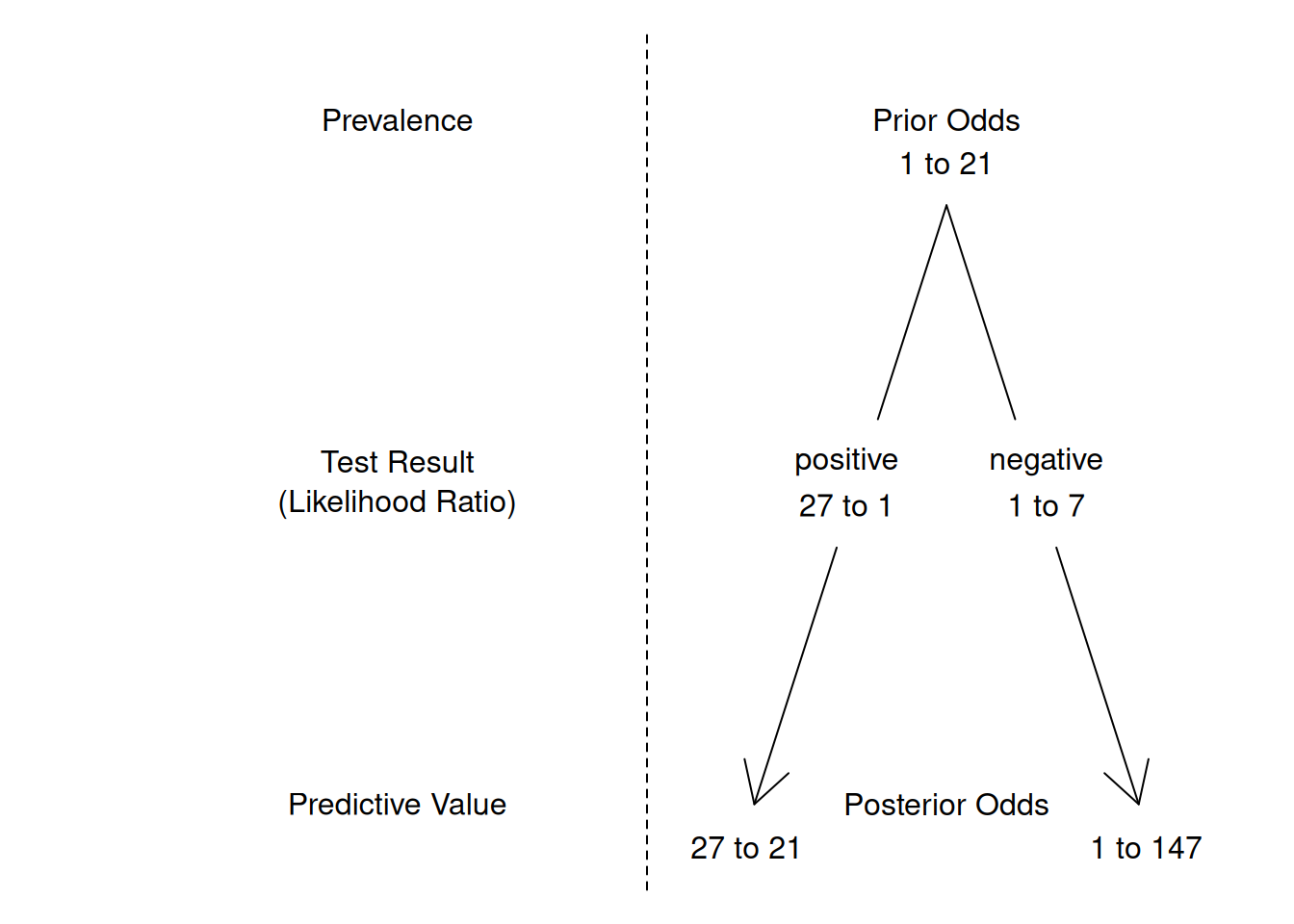
Figure 1.2: Bayesian updating with likelihood ratios. For example, the posterior odds after a positive test result are obtained through multiplication of the prior odds with the positive likelihood ratio: \(\frac{1}{21} \cdot \frac{27}{1} = \frac{27}{21}\).
1.2.5 Diagnostic odds ratio
Definition 1.5 The diagnostic odds ratio
\[\begin{eqnarray} \mbox{DOR} &=& \frac{\Pr(Y=1 \,\vert\,D=1)/\Pr(Y=0 \,\vert\,D=1)}{\Pr(Y=1 \,\vert\,D=0)/\Pr(Y=0 \,\vert\,D=0)} \tag{1.4}\\ &= & \frac{\Pr(D=1 \,\vert\,Y=1)/\Pr(D=0 \,\vert\,Y=1)}{\Pr(D=1 \,\vert\,Y=0)/\Pr(D=0 \,\vert\,Y=0)} \tag{1.5} \end{eqnarray}\]
is a single indicator of test performance. It is defined as the ratio of the odds \(\Pr(Y=1)/\Pr(Y=0)\) of a positive test result in individuals with the disease (\(D=1\)) to the odds of a positive test result in individuals without the disease (\(D=0\)), see Equation (1.4). It can also be written as the ratio of the odds of disease in test positives relative to the odds of disease in test negatives, see Equation (1.5). A higher DOR indicates better diagnostic accuracy, with the test more effectively distinguishing between those with and without the disease.
The diagnostic odds ratio can be calculated as \[ \mbox{DOR} = \frac{\mbox{LR}^+}{\mbox{LR}^-} = \frac{tp \cdot tn}{fp \cdot fn}. \]
In the MW study (Example 1.1) we obtain \[ \mbox{DOR} = \frac{27.1} {0.14} \, = \, 196.5. \]
Figure 1.3 illustrates that the same DOR can be achieved by very different combinations of sensitivity and specificity. For example, a diagnostic test with sensitivity 0.9 and specificity 0.7 will have the same \(\mbox{DOR}=21\) as a test with sensitivity 0.7 and specificity 0.9. The same is true for other summary statistics, such as Youden’s index, which is \(J=0.6\) in both cases.
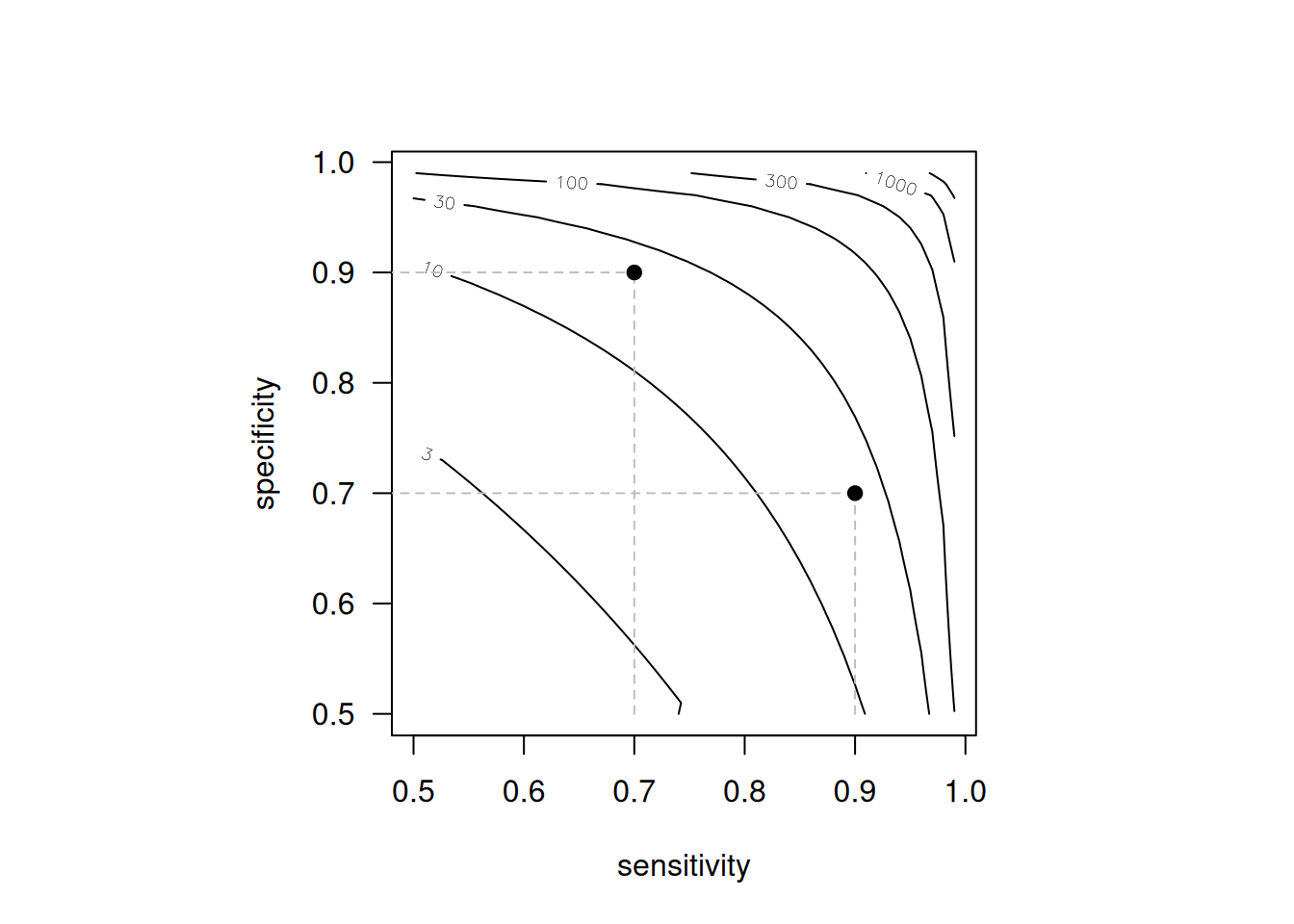
Figure 1.3: Contour plot of the diagnostic odds ratio DOR as a function of sensitivity and specificity. The dots represent a diagnostic test with sensitivity 0.9 and specificity 0.7 and vice versa, where DOR = 21 in both cases.
1.3 Confidence intervals for measures of diagnostic accuracy
So far, we have estimated population parameters using corresponding sample quantities. For instance, sample proportions (p) are used to estimate probabilities (\(\pi\)). These estimates should be reported with a confidence interval (CI) to account for the sample size of the study. Confidence intervals provide a plausible range for the true population values and indicate the impact of sampling variation. However, they do not account for non-sampling errors, such as biases arising from study design, conduct, or analysis.
There are different methods to compute a CI for proportions (e.g. sensitivity, specificity) and ratios (e.g. likelihood ratios). Details on how to construct confidence intervals can be found in Appendix A.
1.3.1 Proportions
Example 1.2 Arroll et al (2003) investigated the diagnostic accuracy of two verbally asked questions for screening for depression in 15 general practices in New Zealand. They report \(tp = 28\) true positives, \(fp = 129\) false positives, \(tn = 263\) true negatives and \(fn = 1\) false negative among \(n=421\) patients in primary care. Overall, 37% (157/421) of the patients screened positive for depression while only 7% (29/421) actually had the disease, according to a subsequent computerised composite international diagnostic interview considered to be the gold standard.
Sensitivity was 97% (95% confidence interval, 83% to 99%) and specificity was 67% (62% to 72%). The likelihood ratio for a positive test was 2.9 (2.5 to 3.4) and the likelihood ratio for a negative test was 0.05 (0.01 to 0.35).
Example 1.3 Kaur et al (2020a) performed a systematic review to assess the diagnostic accuracy of screening tests for early detection of type 2 diabetes and prediabetes in previously undiagnosed adults. Figure 1.4 shows the numbers of true positives, false positives, false negatives, true negatives, sensitivity and specificity (with 95% CI) of 17 studies using HBA1c 6.5% for detecting diabetes.
![Forest plot of HbA1c 6.5\% for detecting diabetes [@Kaur2020_fig].](figures/diabetes-meta.png)
Figure 1.4: Forest plot of HbA1c 6.5% for detecting diabetes (Kaur et al, 2020b).
Wald confidence interval
The standard error of a proportion \(p=x/n\) is \[ \mbox{se}(p) = \sqrt{\frac{p \, (1-p)}{n}}. \]
The 95% error term is defined as \(\mbox{ET}_{95}= 1.96 \cdot \mbox{se}(p)\). The (additive) Wald confidence interval at level 95% then has limits \[ p - \mbox{ET}_{95} \mbox{ and } p + \mbox{ET}_{95}. \]
This confidence interval follows the “add/subtract” construction, because the error term is added to, respectively subtracted from, the estimate \(p\). The factor 1.96 has to be replaced by the appropriate standard normal quantile for other confidence levels. This can be done using the following code:
## [1] 1.644854 1.959964 2.575829Wilson confidence interval
It is usually better to use the Wilson confidence interval, in particular if \(n\) is small or \(p\) is close to 0 or 1. The Wilson interval has better empirical coverage than the Wald interval, as shown in Figure 1.5. Empirical coverage refers to the proportion of times a confidence interval actually contains the true parameter value across many repeated samples. Additionally, the Wilson confidence interval does not have overshoot issues: its limits are always within the unit interval, eliminating the need for truncation.
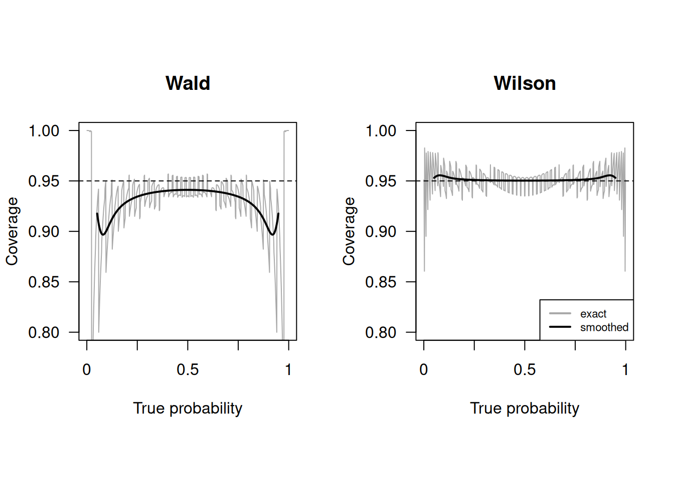
Figure 1.5: Empirical coverage of Wald and Wilson confidence intervals with nominal confidence level \(95\%\) and sample size \(n=50\) (grey line). The solid line is a local average of the coverage, computed as described in Held and Sabanés Bové (2020)
In the MW study (Example 1.1) the Wald and Wilson 95% confidence intervals are obtained using:
##     lower      prop     upper
## 0.8416424 0.8663912 0.8911400## lower prop upper
## 0.8397039 0.8663912 0.8892215The R function prop.test() without continuity correction also
produces a Wilson CI:
## [1] 0.8397039 0.8892215
## attr(,"conf.level")
## [1] 0.95
In Example 1.3 for the first study (Arenata 2010), we obtain the following confidence interval for the specificity:
##     lower      prop     upper
## 0.9560367 0.9682741 0.9805116## lower prop upper
## 0.9535851 0.9682741 0.9784197The limits of the Wald confidence interval are – by construction – symmetric around the observed proportion. The limits of the Wilson interval are shifted slightly to the left.
Other confidence intervals
Other types of confidence intervals can be calculated, for example Agresti, Jeffreys or Clopper-Pearson. Here, we compute the different confidence intervals for the sensitivity in Example 1.2 (screening for depression) based on both questions.
## $p
## [1] 0.9655172
##
## $CIs
##             type     lower     upper
## 1           Wald 0.8991078 1.0000000
## 2         Wilson 0.8282448 0.9938868
## 3        Agresti 0.8110068 1.0000000
## 4       Jeffreys 0.8499223 0.9962538
## 5 ClopperPearson 0.8223557 0.9991274
The upper limit of the Wald confidence interval is actually larger than 1 (“overshoot”): \[ p + \mbox{ET}_{95} = 0.9655172 + 1.96 \cdot \sqrt{(0.9655172 \cdot (1-0.9655172) / 29} = 1.032 \] and in the output truncated to 1. The upper limit of Agresti’s method is also 1. The other methods have an upper limit smaller than one. The method by Clopper-Pearson produces the widest confidence interval. It is often called “exact”, but this is misleading, as it is known to be conservative with too large coverage, see Figure 1.6.
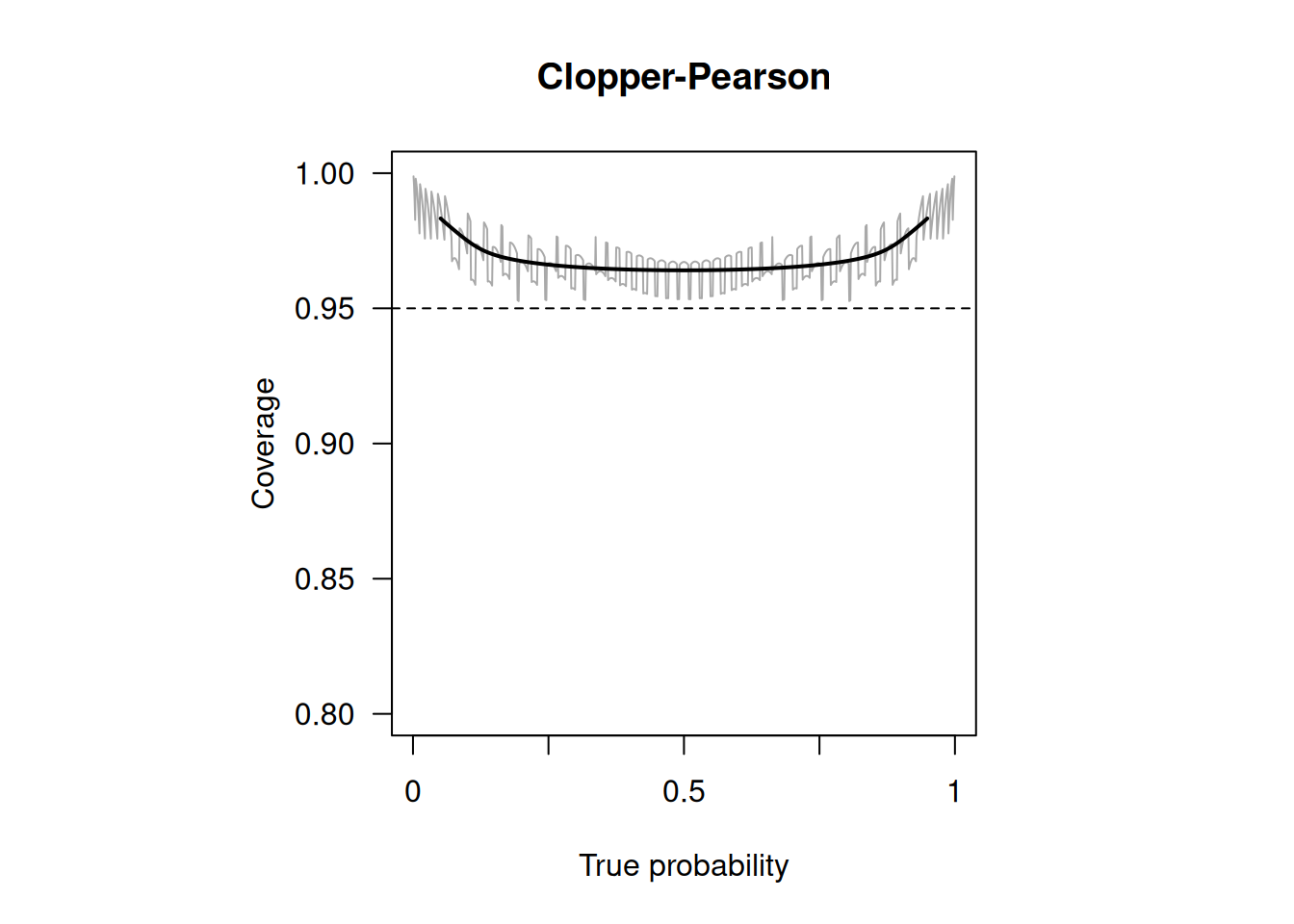
Figure 1.6: Empirical coverage of Clopper-Pearson confidence intervals with nominal confidence level \(95\%\) and sample size \(n=50\) (grey line). The solid line is a local average of the coverage, computed as described in Held and Sabanés Bové (2020)
1.3.2 Likelihood ratios
Likelihood ratios are by definition positive quantities. To avoid overshoot, confidence intervals are therefore constructed on the log-scale. The limits of the 95%-Wald confidence interval for the log positive likelihood ratio \(\log {\mbox{LR}}^+\), for example, are \[ \log {\mbox{LR}}^+ - 1.96 \cdot \mbox{se}(\log {\mbox{LR}}^+) \mbox{ and } \log {\mbox{LR}}^+ + 1.96 \cdot \mbox{se}(\log {\mbox{LR}}^+). \] Note that log always refers to the natural logarithm in this document. Back-transformation to the original scale gives a 95% (multiplicative) Wald confidence interval for the positive likelihood ratio \({\mbox{LR}}^+\) with limits \[ {\mbox{LR}}^+/\mbox{EF}_{.95} \mbox{ and } {\mbox{LR}}^+ \cdot \mbox{EF}_{.95} \] where
\[\mbox{EF}_{.95} =\exp\left\{1.96 \cdot \mbox{se}(\log {\mbox{LR}}^+)\right\}\] is called the 95% error factor (EF). This confidence interval follows the “multiply/divide” construction, as the estimate is multiplied, respectively divided, by the error factor. There are many other confidence intervals in biostatistics that are of the “multiply/divide” type, for example confidence intervals for risk ratios, odds ratios and hazard ratios.
The exact procedure to calculate a 95% confidence interval for a likelihood ratio is as follows, see Table 1.2 for notation:
Calculate standard error on the log scale: \[\begin{eqnarray*} \mbox{se}(\log {\mbox{LR}}^+) & = & \sqrt{\frac{1}{{fp}}-\frac{1}{n_0} +\frac{1}{{tp}}-\frac{1}{n_1}} \\ \mbox{se}(\log {\mbox{LR}}^-) & = & \sqrt{\frac{1}{{tn}}-\frac{1}{n_0} +\frac{1}{{fn}}-\frac{1}{n_1}} \\ \end{eqnarray*}\]
Compute 95% error factor (EF)
The 95% confidence interval for \({\mbox{LR}}^+\) then has limits \[{\mbox{LR}}^+/\mbox{EF}_{.95} \mbox{ and } {\mbox{LR}}^+ \cdot \mbox{EF}_{.95}\]
A 95% confidence interval for \({\mbox{LR}}^-\) is computed accordingly using the standard error \(\mbox{se}(\log {\mbox{LR}}^-)\) for a negative test result.
1.3.3 Diagnostic odds ratio
The confidence interval for the diagnostic odds ratio is also of the “multiply/divide” type, again see Table 1.2 for notation. The steps are:
- Calculate the standard error on the log scale:
\[\begin{eqnarray*} \mbox{se}(\log {\mbox{DOR}}) & = & \sqrt{\frac{1}{{tp}}+\frac{1}{fp}+\frac{1}{{tn}}+\frac{1}{fn}} \\ \end{eqnarray*}\]
Compute the 95% error factor (EF): \[\mbox{EF}_{.95} =\exp\left\{1.96 \cdot \mbox{se}(\log {\mbox{DOR}})\right\}\]
The 95% confidence interval for \({\mbox{DOR}}\) then has limits \[{\mbox{DOR}}/\mbox{EF}_{.95} \mbox{ and } {\mbox{DOR}} \cdot \mbox{EF}_{.95}\]
The function biostatUZH::confIntDiagnostic() computes the estimate and
confidence interval of several indicators of test performance.
For example, for the study on screening for depression (Example 1.2):
##          type    estimate       lower        upper
## 1 Sensitivity  0.96551724 0.828244781   0.99388679
## 2 Specificity  0.67091837 0.622941367   0.71557800
## 3      LRplus  2.93397487 2.507193649   3.43340394
## 4     LRminus  0.05139636 0.007481585   0.35307829
## 5         DOR 57.08527132 7.681345281 424.23925525
## 6         PPV  0.17834395 0.126370172   0.24568228
## 7         NPV  0.99621212 0.978859577   0.99933103
## 8  Prevalence  0.06888361 0.048386233   0.09717738
Alternatively, the computation can be performed with epiR::epi.tests():
  ScreeningData <- as.table(matrix(c(28,129,1,263),
                                   nrow = 2, byrow = TRUE))
  colnames(ScreeningData) <- c("Dis+","Dis-")
  rownames(ScreeningData) <- c("Test+","Test-")
  library(epiR)
  epi.tests(ScreeningData)
## Outcome + Outcome - Total
## Test + 28 129 157
## Test - 1 263 264
## Total 29 392 421
##
## Point estimates and 95% CIs:
## --------------------------------------------------------------
## Apparent prevalence * 0.37 (0.33, 0.42)
## True prevalence * 0.07 (0.05, 0.10)
## Sensitivity * 0.97 (0.82, 1.00)
## Specificity * 0.67 (0.62, 0.72)
## Positive predictive value * 0.18 (0.12, 0.25)
## Negative predictive value * 1.00 (0.98, 1.00)
## Positive likelihood ratio 2.93 (2.51, 3.43)
## Negative likelihood ratio 0.05 (0.01, 0.35)
## False T+ proportion for true D- * 0.33 (0.28, 0.38)
## False T- proportion for true D+ * 0.03 (0.00, 0.18)
## False T+ proportion for T+ * 0.82 (0.75, 0.88)
## False T- proportion for T- * 0.00 (0.00, 0.02)
## Correctly classified proportion * 0.69 (0.64, 0.74)
## --------------------------------------------------------------
## * Exact CIsThe apparent prevalence corresponds to \(\Pr(Y=1)=37\%\), and the true prevalence to \(\Pr(D=1)=7\%\).
1.3.4 Predictive values
If the study follows a cohort design, confidence intervals can be
computed for PPV, NPV and disease prevalence directly from the data. This is what the function epi::epi.tests() always computes. The function biostatUZH::confIntDiagnostic() also computes CIs for PPV and NPV for
a pre-specified prevalence. This approach is based on the following steps:
The limits of a confidence interval for \(\mbox{LR}^+\) (resp. \(\mbox{LR}^-\)) are computed as described in Section 1.3.2.
Multiplication with \({\mbox{Prev}}/({1-\mbox{Prev}})\) gives the limits of a confidence interval for \({\mbox{PPV}/(1-\mbox{PPV})}\) resp. \({(1-\mbox{NPV})/\mbox{NPV}}\) according to equation (1.2), resp. (1.3).
Confidence intervals for \(\mbox{PPV}\) resp. \(\mbox{NPV}\) can be obtained by the usual transformation of the limits obtained in step 2. to the probability scale.
In the screening for depression study (Example 1.2), the predictive values for a prevalence of \(10\%\) are:
##          type    estimate       lower       upper
## 1 Sensitivity  0.96551724 0.828244781   0.9938868
## 2 Specificity  0.67091837 0.622941367   0.7155780
## 3      LRplus  2.93397487 2.507193649   3.4334039
## 4     LRminus  0.05139636 0.007481585   0.3530783
## 5         DOR 57.08527132 7.681345281 424.2392552
## 6         PPV  0.24585060 0.217880547   0.2761435
## 7         NPV  0.99432172 0.962250044   0.9991694
## 8  Prevalence  0.10000000          NA          NA
The assumed prevalence of 10% is higher than the prevalence in the data (6.8%), the positive predictive value is therefore larger and the negative predictive value is smaller.
1.4 Comparing two diagnostic tests
The accuracy of two tests \(A\) and \(B\) for the diagnosis of the same disease can be compared with ratios of probabilities or ratios of likelihood ratios. These ratios are equal to 1 (the reference value), if there is no difference in accuracy between the two tests.
Definition 1.6 The relative sensitivity of test \(A\) vs. test \(B\) is \[\mbox{rSens} = \mbox{Sens}_A / \mbox{Sens}_B\] and the relative specificity is \[\mbox{rSpec} = \mbox{Spec}_A / \mbox{Spec}_B.\] The relative positive likelihood ratio of test \(A\) vs. test \(B\) is \[\mbox{rLR}^+ = \mbox{LR}^+_A / \mbox{LR}^+_B\] and the relative negative likelihood ratio is \[\mbox{rLR}^- = \mbox{LR}^-_A / \mbox{LR}^-_B.\]
Standard errors and confidence intervals can also be computed, but the study design (unpaired or paired) has to be taken into account in the calculations.
Example 1.4 Data from a (hypothetical) randomized unpaired study of early amniocentesis (EA) versus chorionic villus sampling (CVS) for the diagnosis of fetal abnormality is shown in Table 1.5.
| Test | \(Y=0\) | \(Y=1\) | Total | \(Y=0\) | \(Y=1\) | Total |
|---|---|---|---|---|---|---|
| EA | 6 | 116 | 122 | 4844 | 34 | 4878 |
| CVS | 13 | 111 | 124 | 4765 | 111 | 4876 |
The sensitivity and specificity are \(\mbox{Sens}=116/122=95.1\)% and \(\mbox{Spec}=4844/4878=99.3\)% for EA and \(\mbox{Sens}=111/124=89.5\)% and \(\mbox{Spec}=4765/4876=97.7\)% for CVS. Hence,
\[\begin{eqnarray*} \mbox{rSens} & = & 95.1\%/89.5\% = 1.06 \mbox{ and}\\ \mbox{rSpec} & = & 99.3\%/97.7\% = 1.02. \end{eqnarray*}\] We see that the sensitivity of EA is 6% larger than the sensitivity of CVS. The specificity of EA is 2% increased compared to CVS.
The relative sensitivity, specificity, LR\(^{+}\) and LR\(^{-}\), together
with the corresponding confidence intervals, can be computer using the function
biostatUZH::confIntIndependentDiagnostic():
fetAb.tp <- c(116, 111)
fetAb.fp <- c(34, 111)
fetAb.tn <- c(4844, 4765)
fetAb.fn <- c(6, 13)

## T1 (EA) versus T2 (CVS)
print(confIntIndependentDiagnostic(tp = fetAb.tp, fp = fetAb.fp,
                                   t = fetAb.tn, fn = fetAb.fn,
                                   names = c("EA", "CVS"),
                                   conf.level = 0.95))
## type estimateEA estimateCVS ratio lower
## 1 Sens 9.508197e-01 0.8951613 1.0621769 0.9878900
## 2 Spec 9.930299e-01 0.9772354 1.0161624 1.0112088
## 3 LRplus 1.364147e+02 39.3225806 3.4691176 2.3512839
## 4 LRminus 4.952552e-02 0.1072809 0.4616434 0.1813247
## 5 DOR 2.754431e+03 366.5384615 7.5147131 2.5683027
## upper
## 1 1.142050
## 2 1.021140
## 3 5.118385
## 4 1.175321
## 5 21.987639There is some evidence that EA has a better specificity and LR\(^+\) than CVS, since the corresponding confidence intervals do not include the reference value of 1.
Example 1.5 Roldán Nofuentes et al (2012) show the data of a clinical trial carried out at the University Clinic Hospital in Granada, Spain. In this study, two diagnostic tests (T1 and T2) have been applied to 548 males to detect coronary heart disease. The data is paired, that is, each subject performs both tests.
The results for the diseased (Dis) and non-diseased (nonDis) males
are as follows:
##     T1- T1+
## T2-  36  17
## T2+   7 152
## T1- T1+
## T2- 290 10
## T2+ 11 25The function biostatUZH::confIntPairedDiagnostic()can be used in this case:
# Estimates for T1 vs T2
print(confIntPairedDiagnostic(diseased=Dis, nonDiseased=nonDis,
                              names = c("T1", "T2"), conf.level = 0.95))
## type estimateT1 estimateT2 ratio lower
## 1 Sens 0.7971698 0.7500000 1.0628931 1.0024225
## 2 Spec 0.8958333 0.8928571 1.0033333 0.9737883
## 3 LRplus 7.6528302 7.0000000 1.0932615 0.8431956
## 4 LRminus 0.2264151 0.2800000 0.8086253 0.6598383
## 5 DOR 33.8000000 25.0000000 1.3520000 0.3959492
## upper
## 1 1.1270115
## 2 1.0337748
## 3 1.4174891
## 4 0.9909624
## 5 4.6165113There is some evidence that T1 performs better than T2 in terms of sensitivity and LR\(^{-}\), since the corresponding confidence intervals do not include the reference value of 1.
Quite often, in practice, we just use the McNemar test for sensitivity analysis for paired data.
Example 1.6 In Barnell et al (2023), data from 8920 eligible participants are collected for evaluating sensitivity and specificity of two noninvasive tests for colorectal cancer screening. Among 8920 participants, 36 had colorectal cancer. Each participant was tested both by the multi-target stool RNA test (mt-sRNA) and the fecal immunochemical test (FIT), which means, test results are paired within individuals.
To perform McNemar test, we use the mcnemar.test function on the matched data from the two tests.
##      FIT- FIT+
## RNA-    2    0
## RNA+ 6 28##
## McNemar's Chi-squared test with continuity correction
##
## data: CC
## McNemar's chi-squared = 4.1667, df = 1, p-value =
## 0.04123In the paper, the authors report the uncorrected p-value from the test:
##
##  McNemar's Chi-squared test
##
## data:  CC
## McNemar's chi-squared = 6, df = 1, p-value = 0.01431
A p-value of 0.01 suggests that the mt-sRNA test showed significant improvement in sensitivity for colorectal cancer compared with results of the FIT.
1.5 Additional references
Bland (2015) discusses sensitivity and specificity in Chapter 20.6 and standard errors and confidence intervals for a proportion in Chapter 8.4. Likelihood ratios are discussed in Deeks and Altman (2004). A comprehensive account of statistical aspects of binary diagnostic tests can be found in Pepe (2003) (Chapter 2). Altman et al (2000) discuss the relevant confidence intervals in Chapter 6 and 10. Glas et al (2003) discuss properties of the diagnostic odds ratio in detail. Arroll et al (2003) is an example of a study where the methods from this chapter are used in practice. The “Statistics Notes” by Douglas G. Altman and Martin Bland, and sometimes also other co-authors, discuss these methods in a concise and practical way. For this chapter, these are Douglas G. Altman and Bland (1994a), Douglas G. Altman and Bland (1994b), and Deeks and Altman (2004).