Chapter 7 Analysis of continuous outcomes
Effect size estimates quantify clinical relevance, confidence intervals indicate the (im)precision of the effect size estimates as population values, and \(P\)-values quantify statistical significance, i.e. the evidence against the null hypothesis. All three should be reported for each outcome of an RCT and the reported \(P\)-value should be compatible with the selected confidence interval. Binary outcomes are discussed in Chapter 8.
Example 7.1 The Didgeridoo study (Puhan et al, 2005) is a randomized controlled trial with simple randomization. Patients with moderate obstructive sleep apnoea syndrome have been randomized to 4 months of Didgeridoo practice (\(m = 14\)) or 4 months on the waiting list (\(n = 11\)). The primary endpoint is the Epworth scale (integers from 0-24). This scale is ordinal but for the analysis, it is considered continuous due to the large number of possible values. Measurements are taken at the start of the study (Baseline) and after four months (Follow-up). Figure 7.1 compares the follow-up measurements of the treatment and control groups for the primary endpoint.
## treatment
##    Control Didgeridoo
##         11         14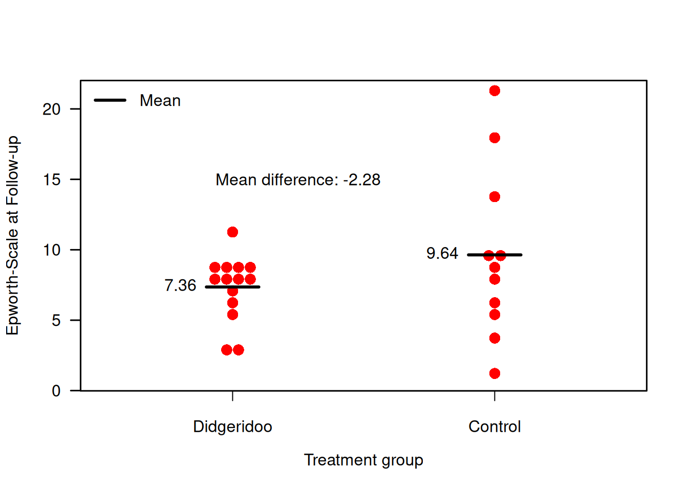
Figure 7.1: Follow-up measurements of primary endpoint in the Didgeridoo Study.
7.1 Comparison of follow-up measurements
7.1.1 \(t\)-test
In order to compare the follow-up measurements between the two groups, a \(t\)-test can be performed. In a \(t\)-test, data are assumed to be normally distributed, and the measurements in the two groups to be independent: with mean \(\mu_T\), variance \(\sigma^2_T\) and sample size \(m\) in the treatment group, and with mean \(\mu_C\), variance \(\sigma^2_C\) and sample size \(n\) in the control group. The quantity of interest is the mean difference \(\Delta = \mu_T - \mu_C\). The variances are assumed to be equal in the two groups, i.e. \(\sigma^2_T = \sigma^2_C = \sigma^2\).
The null hypothesis of a \(t\)-test is \[ H_0: \Delta = 0 . \] The estimate \(\widehat\Delta\) of \(\Delta\) is the difference in sample means. The \(t\)-test statistic is \[ T = \frac{\widehat\Delta}{\mathop{\mathrm{se}}(\widehat\Delta)}, \] with \[ \mathop{\mathrm{se}}(\widehat\Delta) = s \cdot \sqrt{\frac{1}{m} + \frac{1}{n}}, \] where \(s^2\) is the pooled estimate of the variance \(\sigma^2\): \[ s^2 = \frac{(m - 1)s^2_T + (n-1)s^2_C}{m + n - 2}. \] Here \(s^2_T\) and \(s^2_C\) are the sample variances in the two groups. Under the null hypothesis of no effect, the test statistic T follows a \(t\)-distribution with \(m + n - 2\) degrees of freedom (df). For large degrees of freedom, the \(t\)-distribution is close to a standard normal distribution, as illustrated in Figure 7.2.
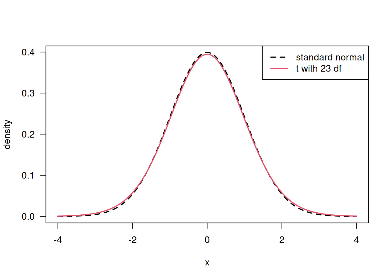
Figure 7.2: Comparison of \(t\)-distribution (with large degree of freedom) to a standard normal distribution.
Let us now apply the \(t\)-test to the follow-up measurements in Example 7.1.
##
##  Two Sample t-test
##
## data:  f.up by treatment
## t = 1.3026, df = 23, p-value = 0.2056
## alternative hypothesis: true difference in means between group Control and group Didgeridoo is not equal to 0
## 95 percent confidence interval:
##  -1.340366  5.898807
## sample estimates:
##    mean in group Control mean in group Didgeridoo
## 9.636364 7.357143## [1] 2.279221There is no evidence for a difference in follow-up means (\(P\)-value = 0.21). The \(t\)-test gives identical results as a linear regression analysis:
# regression analysis
library(biostatUZH)
model1 <- lm(f.up ~ treatment)
knitr::kable(tableRegression(model1, intercept=FALSE,
latex = FALSE, xtable = FALSE))| Coefficient | 95%-confidence interval | \(p\)-value | |
|---|---|---|---|
| treatmentDidgeridoo | -2.28 | from -5.90 to 1.34 | 0.21 |
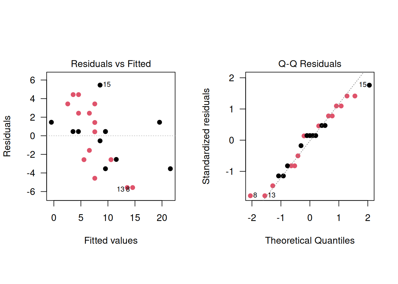
The advantages of the regression analysis are that it can easily be generalized and that the residuals can be checked. In the Didgeridoo study, the regression diagnostics indicate a poor model fit, with signs of variance heterogeneity:
par(mfrow=c(1,2), pty="s", las=1)
plot(model1, which=1, pch=19, col=treatment)
plot(model1, which=2, pch=19, col=treatment)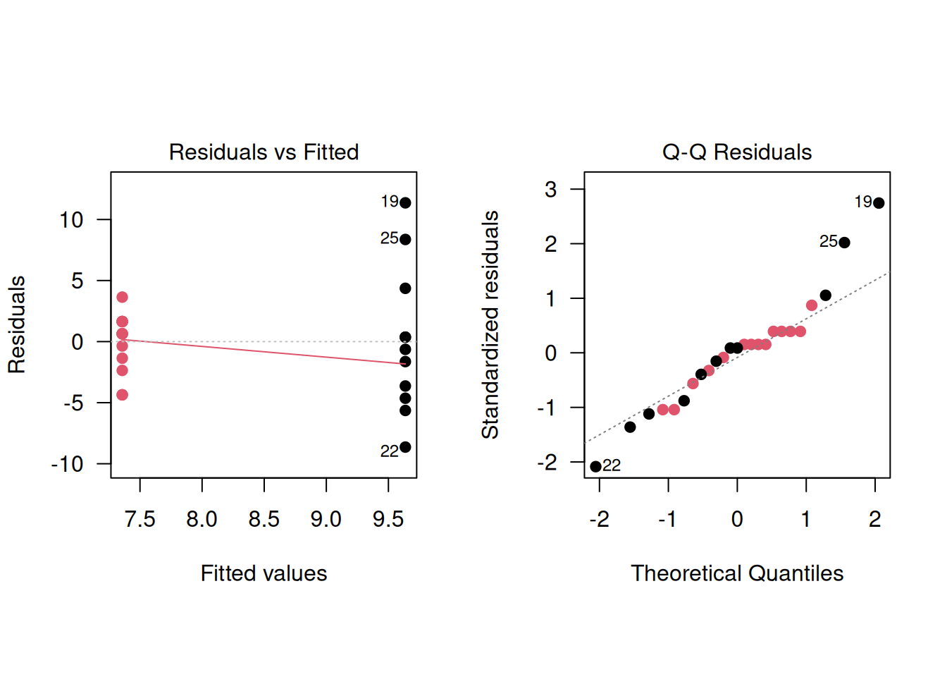
Bartlett’s test can be used to test the equality of variance,
using the R function bartlett.test():
##
##  Bartlett test of homogeneity of variances
##
## data:  f.up by treatment
## Bartlett's K-squared = 9.1295, df = 1, p-value =
## 0.002515
The test indicates strong evidence for variance heterogeneity (\(p=0.003\)), which confirms the earlier findings based on regression diagnostics. However, it is not recommended to pre-test for equal variances and then choose between a \(t\)-test or Welch’s test. Such a two-stage procedure fails to control the Type-I error rate and usually makes the situation worse, see Zimmerman (2004).
7.1.2 Welch’s test
In the case of unequal variances, \(\sigma_T^2\) and \(\sigma^2_C\) are assumed to be different and the standard error of \(\widehat\Delta\) then is
\[\begin{equation*}
\mbox{se}(\widehat \Delta) = \sqrt{\frac{s_T^2}{m} + \frac{s_C^2}{n}},
\end{equation*}\]
where \(s_T^2\) and \(s_C^2\) are estimates of the variances \(\sigma_T^2\) and
\(\sigma_C^2\) in the two groups. In this case, the exact null distribution of
\(T=\widehat \Delta/{\mbox{se}(\widehat \Delta)}\) is unknown.
Welch’s test is an appropriate solution, and the default in t.test(),
since it is not recommended to pre-test for equal variances and then choose between a t-test or Welch’s test (two-stage procedure).
This test can have non-integer degrees of freedom.
##
##  Welch Two Sample t-test
##
## data:  f.up by treatment
## t = 1.187, df = 12.381, p-value = 0.2575
## alternative hypothesis: true difference in means between group Control and group Didgeridoo is not equal to 0
## 95 percent confidence interval:
##  -1.890289  6.448731
## sample estimates:
##    mean in group Control mean in group Didgeridoo
##                 9.636364                 7.357143
There is no evidence for a difference in follow-up means (\(p = 0.26\))
7.2 Analysis of baseline and follow-up measurements
In the previous section, we focused solely on follow-up measurements. Now, we consider both baseline and follow-up measurements in the analysis.
7.2.1 Change scores
Baseline values may be imbalanced between treatment groups just as any other prognostic factor. To analyse change from baseline, we use change scores:
Definition 7.1 The change score is the change from baseline defined as: \[ \mbox{change score} = \mbox{follow-up} - \mbox{baseline}. \]
Example 7.1 (continued) Figure 7.3 shows the combinations of baseline and follow-up measurements for each individual. It is visible that the change from baseline to follow-up is larger in the treatment group than in the control group. Figure 7.4 now directly compares the change scores.
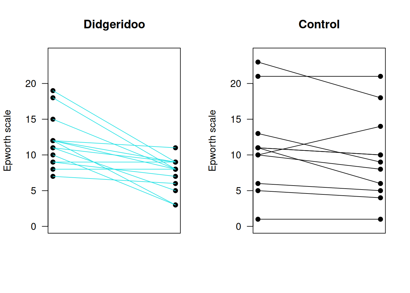
Figure 7.3: Individual baseline and follow-up measurements in the Didgeridoo Study by treatment group.
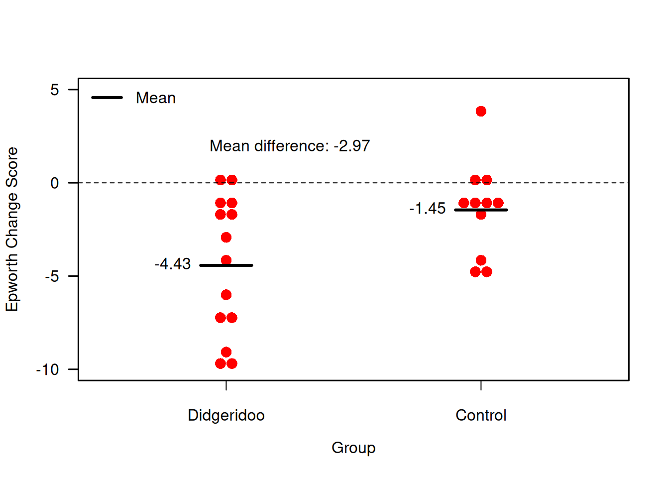
Figure 7.4: Change scores for primary endpoint in the Didgeridoo Study.
A change score analysis for the Didgeridoo study using a \(t\)-test yields:
##
##  Two Sample t-test
##
## data:  change.score by treatment
## t = 2.2748, df = 23, p-value = 0.03256
## alternative hypothesis: true difference in means between group Control and group Didgeridoo is not equal to 0
## 95 percent confidence interval:
##  0.2695582 5.6784938
## sample estimates:
##    mean in group Control mean in group Didgeridoo
## -1.454545 -4.428571## [1] 2.974026There is hence evidence for a difference in mean change score between the two groups (\(p = 0.033\)).
The change score analysis can also be done with a regression model:
# Change score analysis
model2 <- lm(f.up ~ treatment + offset(baseline))
knitr::kable(tableRegression(model2, intercept=FALSE,
latex = FALSE, xtable = FALSE))| Coefficient | 95%-confidence interval | \(p\)-value | |
|---|---|---|---|
| treatmentDidgeridoo | -2.97 | from -5.68 to -0.27 | 0.033 |
The offset(x) command fixes the coefficient of x at 1.
The regression diagnostics show a somewhat better model fit:
As a sensitivity analysis, other tests can be applied:
- Welch’s test,
- Behren’s test, using
biostatUZH::behrens.test(), which can be derived with Bayesian arguments, - Mann Whitney test, a nonparametric alternative,
- Permutation test, which follows the randomization model approach.
Adjustments for covariates are not standard with all these methods.
Welch’s and Behrens’ tests
Both Welch’s and Behren’s test indicate evidence for a difference in mean change score:
##
##  Welch Two Sample t-test
##
## data:  change.score by treatment
## t = 2.3731, df = 22.782, p-value = 0.02646
## alternative hypothesis: true difference in means between group Control and group Didgeridoo is not equal to 0
## 95 percent confidence interval:
##  0.3802133 5.5678387
## sample estimates:
##    mean in group Control mean in group Didgeridoo
## -1.454545 -4.428571##
## Behrens' t-test
##
## data: change.score by treatment
## t = 2.2825, df = 19, p-value = 0.03415
## alternative hypothesis: true difference in means between group Control and group Didgeridoo is not equal to 0
## 95 percent confidence interval:
## 0.2469164 5.7011356
## sample estimates:
## mean in group Control mean in group Didgeridoo
## -1.454545 -4.428571Mann-Whitney test
Mann-Whitney test gives a confidence interval for the median of the
difference between a sample from the Didgeridoo and the control
group (difference in location), which is hard to interpret:
##
##  Wilcoxon rank sum test with continuity correction
##
## data:  change.score by treatment
## W = 111.5, p-value = 0.06003
## alternative hypothesis: true location shift is not equal to 0
## 95 percent confidence interval:
##  -3.206331e-05  5.999997e+00
## sample estimates:
## difference in location
##               2.000053
Mann-Whitney test has fewer assumptions than the \(t\)-test, but also less power.
Permutation test
An alternative method to compute a \(P\)-value is the permutation test based on the randomisation model. The idea is that, under the null hypothesis \(H_0\), the mean difference does not depend on the treatment allocation. The distribution of the mean difference under \(H_0\) is derived under all possible permutations of treatment allocation. The comparison with the observed difference then gives a \(P\)-value. In practice, a Monte Carlo random sample is taken from all possible permutations. This approach can be extended to stratified randomisation, etc. Figure 7.5 illustrated the permutation test for the change score analysis. Note that in total, there are \({25 \choose 14} \approx 4.5\) Mio. distinct permutations of treatment allocation.
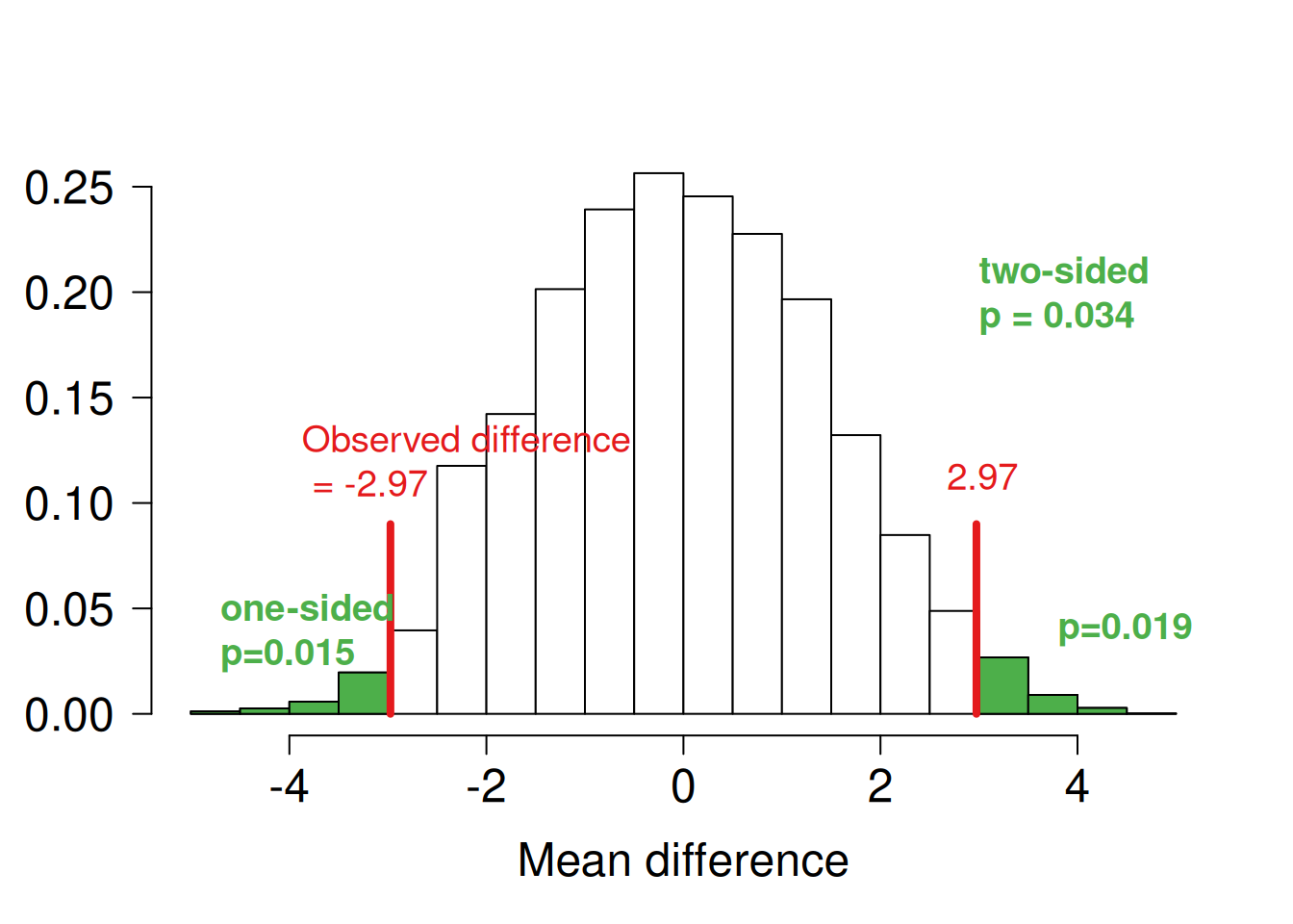
Figure 7.5: Mean difference in change score analysis based on 10000 random permutations
Summary of sensitivity analysis
| Method | p-value | 95% confidence interval |
|---|---|---|
| t-test | 0.033 | 0.27 to 5.68 |
| Welch’s test | 0.026 | 0.38 to 5.57 |
| Behrens’ test | 0.034 | 0.25 to 5.70 |
| Mann-Whitney test | 0.06 | 0.00 to 6.00 |
| Permutation test | 0.034 | 0.16 to 5.84 |
The question now is: which test to choose? The statistical analysis should be pre-specified in the analysis plan, and the other results reported as sensitivity analyses.
Comparison of effect estimates
Let us now define some notation. The outcome means
- at Baseline in both groups is \(\mu_B\),
- at Follow-up in the control group is \(\mu\), and
- at Follow-up in the treatment group is \(\mu + \Delta\).
The mean difference \(\Delta\) is of primary interest. We assume a common variance \(\sigma^2\) of all measurements, and \(n\) observations in each group. The correlation between baseline and follow-up measurements is defined as \(\rho\). The estimated difference of mean follow-up measurements is denoted by \(\widehat\Delta_1\) and the estimated difference of mean change scores by \(\widehat\Delta_2\). Both estimates are unbiased (assuming baseline balance).
The variance of these estimates is \(\mathop{\mathrm{Var}}(\widehat\Delta_1) = 2\sigma^2/n\) and \(\mathop{\mathrm{Var}}(\widehat\Delta_2) = 4\sigma^2(1 - \rho)/n\), respectively. The estimate \(\widehat\Delta_2\) will thus have smaller variance than \(\widehat\Delta_1\) for \(\rho > 1/2\), so it will produce narrower confidence intervals and more powerful tests. In the Didgeridoo study, the estimated correlation \(\hat \rho = 0.72\).
7.2.2 Analysis of covariance
Analysis of covariance (ANCOVA) is an extension of the change score analysis:
model3 <- lm(f.up ~ treatment + baseline)
knitr::kable(tableRegression(model3, intercept = FALSE,
latex = FALSE, xtable = FALSE))| Coefficient | 95%-confidence interval | \(p\)-value | |
|---|---|---|---|
| treatmentDidgeridoo | -2.74 | from -5.14 to -0.35 | 0.027 |
| baseline | 0.67 | from 0.42 to 0.92 | < 0.0001 |
Now the coefficient of baseline is estimated from the data.
The regression diagnostics indicate a good model fit:
par(mfrow=c(1,2), pty="s", las=1)
plot(model3, which=1, pch=19, col=treatment, add.smooth=FALSE)
plot(model3, which=2, pch=19, col=treatment)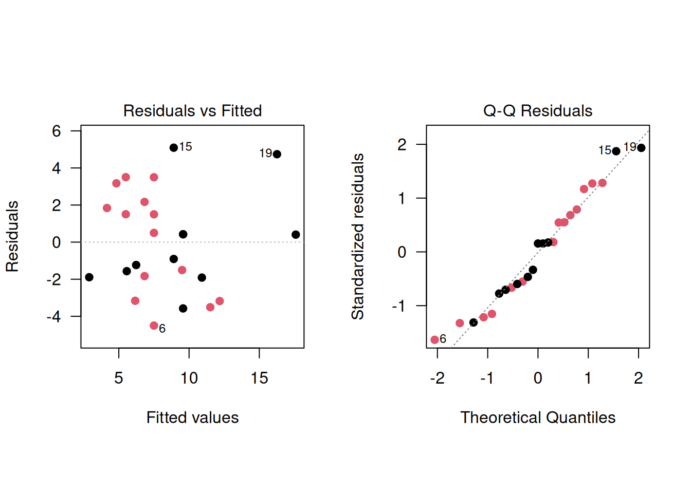
Let us denote the coefficient of the baseline variable as \(\beta\). The ANCOVA model reduces to the analysis of follow-up for \(\beta = 0\), and to the analysis of change scores for \(\beta = 1\). The ANCOVA model estimates \(\beta\) and the mean difference \(\Delta\) jointly with multiple regression. The estimate \(\hat\beta\) is usually close to the correlation \(\rho\).
Example 7.1 (continued) Comparison of the three different analysis methods in the Didgeridoo study:
# Follow-up analysis
knitr::kable(tableRegression(model1, intercept=FALSE,
latex = FALSE, xtable = FALSE))| Coefficient | 95%-confidence interval | \(p\)-value | |
|---|---|---|---|
| treatmentDidgeridoo | -2.28 | from -5.90 to 1.34 | 0.21 |
# Change score analysis
model2 <- lm(f.up ~ treatment + offset(baseline))
knitr::kable(tableRegression(model2, intercept=FALSE,
latex = FALSE, xtable = FALSE))| Coefficient | 95%-confidence interval | \(p\)-value | |
|---|---|---|---|
| treatmentDidgeridoo | -2.97 | from -5.68 to -0.27 | 0.033 |
# ANCOVA
model3 <- lm(f.up ~ treatment + baseline)
knitr::kable(tableRegression(model3, intercept = FALSE,
latex = FALSE, xtable = FALSE))| Coefficient | 95%-confidence interval | \(p\)-value | |
|---|---|---|---|
| treatmentDidgeridoo | -2.74 | from -5.14 to -0.35 | 0.027 |
| baseline | 0.67 | from 0.42 to 0.92 | < 0.0001 |
Conditioning on baseline values
Let \(\bar {b}_T\) and \(\bar {b}_C\) denote the observed mean baseline values in the current trial. The expectation of \(\widehat\Delta_1\) and \(\widehat\Delta_2\) given \(\bar b_T\) and \(\bar b_C\), are
\[\begin{eqnarray*} \mathop{\mathrm{\mathsf{E}}}(\widehat \Delta_1 \,\vert\,\bar {b}_T, \bar {b}_C) & = & \Delta + \underbrace{\rho \cdot (\bar b_T - \bar b_C)}_{\color{red}{bias}} \\ \mathop{\mathrm{\mathsf{E}}}(\widehat \Delta_2 \,\vert\,\bar {b}_T, \bar {b}_C) & = & \Delta + \underbrace{(\rho - 1) \cdot (\bar b_T - \bar b_C)}_{\color{red}{bias}} \\ \end{eqnarray*}\]
Hence both \(\widehat\Delta_1\) and \(\widehat\Delta_2\) given \(\bar b_T\) and \(\bar b_C\) are biased if there is correlation \(\rho > 0\) between baseline and follow-up measurements and there is baseline imbalance (\(\bar b_T \neq \bar b_C\)).
In the Didgeridoo study there is some baseline imbalance: \(\bar {b}_T=11.1\), \(\bar {b}_C=11.8\).
In contrast, the ANCOVA estimate \(\widehat \Delta_3\) is an unbiased estimate of the mean difference \(\Delta\) with variance
\[ \mathop{\mathrm{Var}}(\widehat \Delta_3) = 2 \sigma^2(1-\rho^2)/n, \] which is always smaller than the variances of \(\widehat \Delta_1\) and \(\widehat \Delta_2\). This means that the treatment effect estimate has a smaller standard error. As a result, the required sample size for ANCOVA reduces by the factor \(\rho^2\) compared to the standard comparison of two groups without baseline adjustments.
The variances of the effect estimates in the three models can be compared by the corresponding variance factors:
\[ \mathop{\mathrm{Var}}(\widehat \Delta) = \color{red}{\mbox{variance factor}} \cdot \sigma^2 /n \]
\[ \begin{aligned} \mathop{\mathrm{Var}}(\widehat \Delta_1) &= \color{red}{2} \cdot \sigma^2 /n \\ \mathop{\mathrm{Var}}(\widehat \Delta_2) &= \color{red}{4 (1-\rho)} \cdot \sigma^2 /n \\ \mathop{\mathrm{Var}}(\widehat \Delta_3) &= \color{red}{2 (1-\rho^2)} \cdot \sigma^2/n \end{aligned} \]
Figure 7.6 compares the variance factors of the three models for varying correlations \(\rho\).
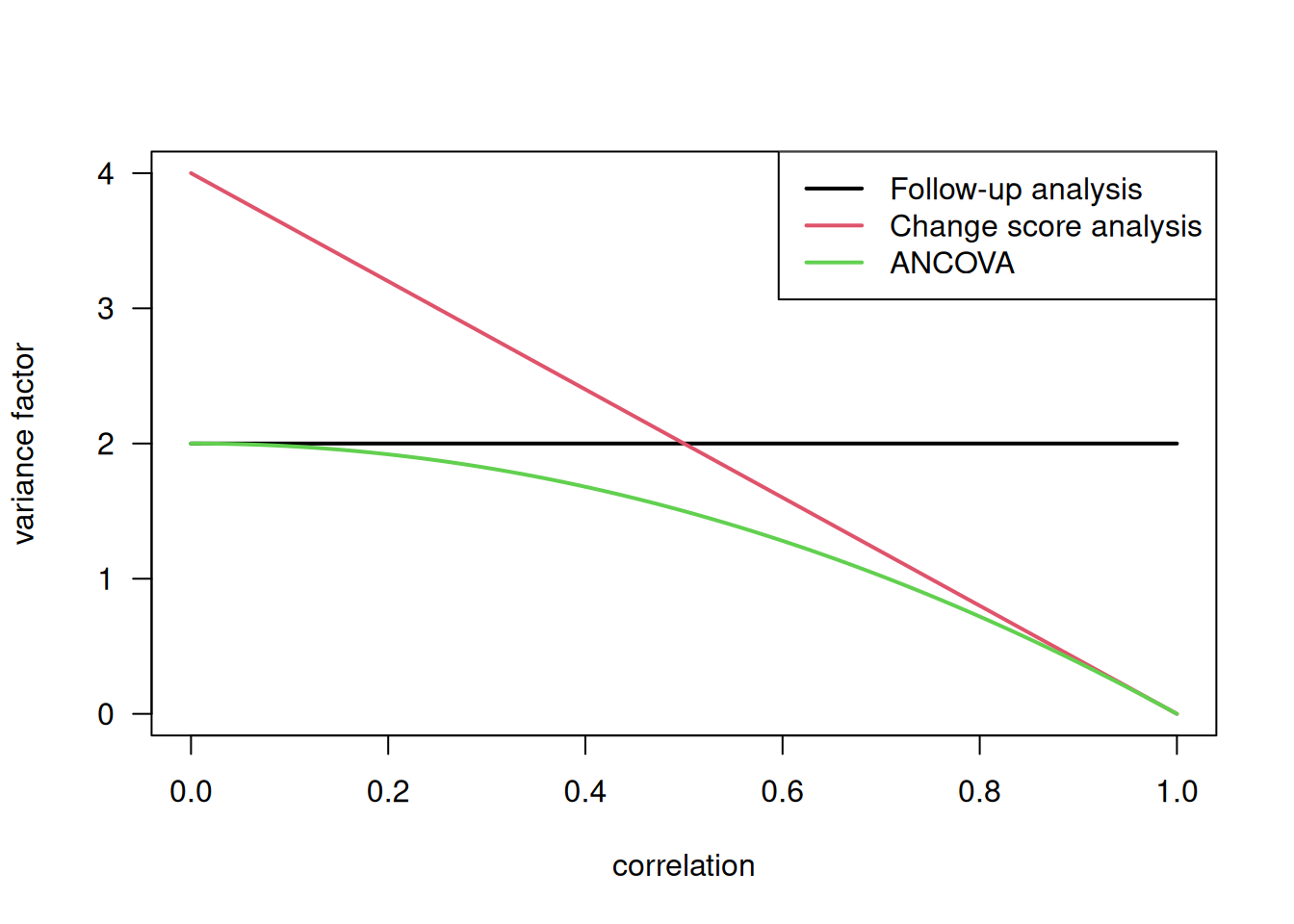
Figure 7.6: Comparison of variance factors
Least-squares means
We have seen in the previous section that the ANCOVA estimate is
different from the difference of the raw mean change scores. This may
cause confusion in tables reporting results from RCTs, if both raw means
of change are reported together with the ANOVA estimate of the
difference. An alternative is to report adjusted least-squares (LS)
means via fitted values in both groups, which are compatible with the
ANCOVA estimate. Computation is illustrated with the lsmeans package
##  treatment  baseline prediction    SE df
##  Control        11.5      10.03 0.978 23
##  Didgeridoo     11.5       7.05 0.867 23
## treatment baseline prediction SE df
## Control 11.5 9.90 0.863 22
## Didgeridoo 11.5 7.15 0.764 22The raw means rawMeans are simply the means of the follow-up measurements in both groups,
whereas the adjusted least-squares means adjMeans are adjusted for the effect of baseline.
Note that 11.5, the mean baseline value in the dataset,
is the assumed mean baseline value in both groups.
The ANCOVA estimate can now be calculated as the difference of the least-squares means, denoted as
predicted:
\(7.15 - 9.90 = -2.74\).
Adjusting for other variables
ANCOVA allows a wide range of variables measured at baseline to be used to adjust the mean difference. The safest approach to selecting these variables is to decide this before the trial starts (in the study protocol). Prognostic variables used to stratify the allocation should always be included as covariates.
Example 7.1 (continued) In the Didgeridoo study, the mean difference has been adjusted for
severity of the disease (base.apnoea) and for weight change during
the study period (weight.change).
| Coefficient | 95%-confidence interval | \(p\)-value | |
|---|---|---|---|
| treatmentDidgeridoo | -2.75 | from -5.35 to -0.15 | 0.039 |
| baseline | 0.67 | from 0.41 to 0.93 | < 0.0001 |
| weight.change | -0.17 | from -0.92 to 0.57 | 0.63 |
| base.apnoea | 0.023 | from -0.25 to 0.29 | 0.86 |
7.3 Additional references
Relevant references are Chapter 10 “Comparing the Means of Small Samples” and Chapter 15 “Multifactorial Methods” in Bland (2015) as well as Chapter 6 “Analysis of Results” in Matthews (2006). Analysing controlled trials with baseline and follow up measurements is discussed in the Statistics Note from Vickers and Altman (2001). Permutation tests in biomedical research are described in Ludbrook and Dudley (1998). Studies where the methods from this chapter are used in practice are for example Ravaud et al (2009), Porto et al (2011), James et al (2004).