Chapter 12 Crossover trials
Up to now, we have considered parallel group designs. A crossover trial trial compares the outcome of a patient when given treatment A to the outcome from the same patient when given treatment B. This means that participants act as their own controls, which leads to larger precision of the treatment effect. Crossover trials are possible if the aim of therapy is not to cure a condition. A typical application of the crossover design is to compare different pain-relieving drugs. The simplest crossover trial design is the AB/BA design.
12.1 The AB/BA design
The AB/BA design is illustrated in Table 12.1. There are two treatment periods, and patients are randomized into two sequence groups, where patients in group AB receive the treatments in the order A-B, and patients in group BA receive the treatments in the order B-A.
This design ensures that period effects can be separated from treatment effects, which would not be the case if all patients had been allocated to group AB. For example, to study the effect of pain-relieving drugs for headaches, a possible period effect may be due to changes in weather conditions in the two periods. If all patients were treated in the order A-B, then any difference in the outcome between A and B may be due to the period effect alone, or a combination of the period and treatment effect.
| Group | Period 1 | Period 2 |
|---|---|---|
| AB | A | B |
| BA | B | A |
Analysis methods for crossover trials with an AB/BA design are explained in the next sections, first for continuous outcomes and then for binary outcomes.
12.2 Continuous outcomes
The following illustrating example will be used throughout this section.
Example 12.1 The Enuresis Trial (Matthews, 2006) is a placebo-controlled trial on \(n=29\) children suffering from enuresis (bed wetting). In group AB (\(n_{AB}=17\)), the drug is given for 14 days and the outcome (number of dry nights) is recorded. Then, a placebo is administered for a fortnight and the same outcome variable is recorded. In group BA (\(n_{BA}=12\)), first placebo and then the drug is given. The outcome is treated as a continuous variable, although strictly speaking it is a count variable with values between 0 and 14.
##   group id outcome1 outcome2 diff treatment placebo
## 1    AB  1        8        5    3         8       5
## 2    AB  2       14       10    4        14      10
## 3    AB  3        8        0    8         8       0
Patient-level data for group AB and group BA comparing the outcomes under treatment and under placebo for each patient are shown in Figure 12.1 together with the corresponding means.
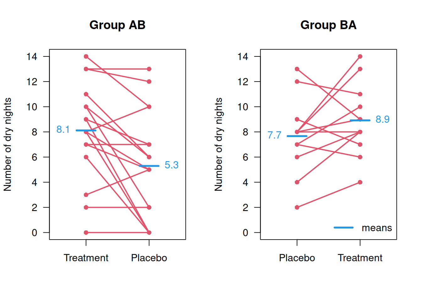
Figure 12.1: Patient-level data from the Enuresis Trial.
12.2.1 Simple analysis
First, we set the notation as follows:
- \(x_{ij}\) is the (continuous) outcome of patient \(i\) in period \(j\), for \(i=1,\ldots, n\),
- \(\alpha\) is the mean outcome in period 1 under placebo (treatment B),
- \(\Delta\) is the treatment effect of the drug relative to placebo,
- \(\beta\) is the period effect of period 2 relative to period 1.
The mean outcomes are therefore modeled as:
| Period | Group AB | Group BA |
|---|---|---|
| 1 | \(\mathop{\mathrm{\mathsf{E}}}(x_{i1}) = \alpha + \Delta\) | \(\mathop{\mathrm{\mathsf{E}}}(x_{i1}) = \alpha\) |
| 2 | \(\mathop{\mathrm{\mathsf{E}}}(x_{i2}) = \alpha + \beta\) | \(\mathop{\mathrm{\mathsf{E}}}(x_{i2}) = \alpha + \Delta + \beta\) |
Now consider the within-patient differences \(d_i = x_{i1} - x_{i2}\) and let \(\bar d_{AB}\) and \(\bar d_{BA}\) denote the mean difference in group AB and group BA, respectively. Then:
\[\begin{eqnarray*} \mathop{\mathrm{\mathsf{E}}}(\bar d_{AB}) & = & \, \, \, \, \Delta - \beta \mbox{ in group AB}\\ \mbox{ and } \mathop{\mathrm{\mathsf{E}}}(\bar d_{BA}) & = & - \Delta - \beta \mbox{ in group BA}, \\ \mbox{ so } \mathop{\mathrm{\mathsf{E}}}(\bar d_{AB} -\bar d_{BA} )& = & 2 \Delta \, . \end{eqnarray*}\]
The null hypothesis of no treatment difference, \(\Delta = 0\), can hence be investigated with an unpaired two-sample \(t\)-test applied to the two sets of within-patient differences. The treatment effect \(\Delta\) is finally estimated as half of the differences in means: \(\hat \Delta = (\bar d_{AB} -\bar d_{BA})/2\).
Example 12.1 (continued) Results of the simple analysis in the Enuresis Trial:
##
##  Two Sample t-test
##
## data:  diff by group
## t = 3.2925, df = 27, p-value = 0.002773
## alternative hypothesis: true difference in means between group AB and group BA is not equal to 0
## 95 percent confidence interval:
##  1.535005 6.612054
## sample estimates:
## mean in group AB mean in group BA
##         2.823529        -1.250000
## [1] 2.036765## confidence interval for treatment effect: divide by 2
(DeltaConfInt <- simpleAnalysis$conf.int/2)## [1] 0.7675023 3.3060271
## attr(,"conf.level")
## [1] 0.95Just for illustration, but not recommended: A naive analysis of the AB/BA design would be to compare differences \(d_i\) of treatment to placebo measurements with a paired \(t\)-test, ignoring group membership: \[ d_i = \left\{ \begin{array}{rl} x_{i1} - x_{i2} & \mbox{ in group AB} \\ x_{i2} - x_{i1} & \mbox{ in group BA} \\ \end{array}\right. \] The mean \(\bar d\) then has expectation \[\begin{eqnarray*} \mathop{\mathrm{\mathsf{E}}}(\bar d) &=& \frac{1}{n_{AB}+n_{BA}} \left\{n_{AB} (\Delta - \beta) + n_{BA} (\Delta + \beta) \right\} \\ & = & \Delta - \beta \, \frac{n_{AB}-n_{BA}}{n_{AB}+n_{BA}}. \end{eqnarray*}\]
The estimate from the t-test is confounded by the period effect \(\beta\). Bias occurs whenever group sizes are unequal (\(n_{AB} \neq n_{BA}\)) and there is a period effect (\(\beta \neq 0\)).
Example 12.1 (continued) Results of the non-recommended paired \(t\)-test in the Enuresis Trial:
##
##  Paired t-test
##
## data:  enuresis$treatment and enuresis$placebo
## t = 3.5265, df = 28, p-value = 0.001471
## alternative hypothesis: true mean difference is not equal to 0
## 95 percent confidence interval:
##  0.9105547 3.4342728
## sample estimates:
## mean difference
## 2.172414## [1] 0.9105547 3.4342728
## attr(,"conf.level")
## [1] 0.95The paired \(t\)-test gives different results and is not recommended.
Between-patient variation
The previously described recommended analysis (unpaired \(t\)-test) also holds if we allow for patient-specific effects \(\xi_i\):
| Period | Group AB | Group BA |
|---|---|---|
| 1 | \(\mathop{\mathrm{\mathsf{E}}}(x_{i1}) = \alpha + \Delta + {\color{red}\xi_i}\) | \(\mathop{\mathrm{\mathsf{E}}}(x_{i1}) = \alpha + {\color{red}\xi_i}\) |
| 2 | \(\mathop{\mathrm{\mathsf{E}}}(x_{i2}) = \alpha + \beta + {\color{red}\xi_i}\) | \(\mathop{\mathrm{\mathsf{E}}}(x_{i2}) = \alpha + \Delta + \beta + {\color{red}\xi_i}\) |
since the \(\xi_i\)’s cancel when we calculate patient-specific differences \(d_{i} = x_{i1} - x_{i2}\). This illustrates that between-patient variation is eliminated in the standard analysis of crossover trials.
12.2.2 Analysis using mixed models
It is also possible to perform an analysis of the original outcomes \(x_{ij}\) using a mixed model with patient-specific random effects \(\xi_i\). This will give the same treatment effect (with confidence interval and \(P\)-value) as the simple analysis based on the unpaired \(t\)-test, but also provides an estimate of the period effect and estimates of within- and between-patient variances.
Example 12.1 (continued) Results in the Enuresis Trial:
# restructuring the data
outcome <- c(enuresis$outcome1, enuresis$outcome2)
n <- nrow(enuresis)
period <- as.factor(c(rep(1, n), rep(2, n)))
id <- c(enuresis$id,enuresis$id)
treatment <- as.numeric(c((enuresis$group=="AB"),
                          (enuresis$group=="BA")))

## fit mixed model in R
library(lme4)
mixed1 <- lmer(outcome ~ period + treatment + (1|id))
print(coef(summary(mixed1)))
## Estimate Std. Error t value
## (Intercept) 6.7370690 0.7709291 8.738896
## period2 -0.7867647 0.6186000 -1.271847
## treatment 2.0367647 0.6186000 3.292539The mixed model gives the same estimate of the treatment effect as the simple analysis based on the comparison of patient-specific differences with an unpaired \(t\)-test, but also provides an estimate of the period effect (\(\hat \beta = -0.79\)).
The approach also gives estimates of the variance (respectively standard deviation) components:
##  Groups   Name        Std.Dev.
##  id       (Intercept) 2.8352
##  Residual             2.3203
The estimated between-patient standard deviation is \(\sigma_b = 2.84\) and the estimated within-patient standard deviation is \(\sigma_w = 2.32\).
12.3 The issue of carryover
The above analysis assumes that there is no carryover effect, i.e. effects of the treatment given in period 1 do not persist during period 2. A statistical approach to handle carryover has been suggested: first, test for carryover, and if significant, compare only data from period 1, otherwise, analyse data from period 1 and 2 jointly assuming there is no carryover effect. We emphasize that this is generally not recommended due to lack of power and other problems.
The recommended approach is not to use a crossover design when there is a possibility of a carryover effect. You should try to use non-statistical arguments, perhaps based on the half-lives of drugs, etc., to decide how long treatment effects are likely to persist and apply appropriate washout periods between the two treatment periods.
12.3.1 Analysis of carryover
Suppose now we have an additional carryover effect \(\gamma\) in period 2 for patients in group AB, but not in group BA:
| Period | Group.AB | Group.BA |
|---|---|---|
| 1 | \(\mathop{\mathrm{\mathsf{E}}}(x_{i1}) = \alpha + \Delta\) | \(\mathop{\mathrm{\mathsf{E}}}(x_{i1}) = \alpha\) |
| 2 | \(\mathop{\mathrm{\mathsf{E}}}(x_{i2}) = \alpha + \beta {\color{red} \,+\, \gamma}\) | \(\mathop{\mathrm{\mathsf{E}}}(x_{i2}) = \alpha + \Delta + \beta\) |
Then:
\[\begin{eqnarray*} \mathop{\mathrm{\mathsf{E}}}(\bar d_{AB}) & = & \, \, \, \, \Delta - \beta {\color{red} \, - \, \gamma} \mbox{ in group AB},\\ \mathop{\mathrm{\mathsf{E}}}(\bar d_{BA}) & = & - \Delta - \beta \mbox{ in group BA}, \\ \mbox{ so } \mathop{\mathrm{\mathsf{E}}}(\bar d_{AB} -\bar d_{BA} )& = & 2 \Delta {\color{red} \, - \, \gamma} \, . \end{eqnarray*}\]
So, for \(\gamma \neq 0\), the traditional estimate of \(\Delta\) will be biased.
12.3.2 Test for carryover
A test for \(H_0\): \(\gamma = 0\) can be performed using a standard \(t\)-test comparing the sums \(s_i=x_{i1} + x_{i2}\) across groups:
\[\begin{eqnarray*} \mathop{\mathrm{\mathsf{E}}}(\bar s_{AB}) & = & 2 \alpha + \Delta + \beta + \gamma \mbox{ in group AB},\\ \mathop{\mathrm{\mathsf{E}}}(\bar s_{BA}) & = & 2 \alpha + \Delta + \beta \mbox{ in group BA}, \\ \mbox{ so } \mathop{\mathrm{\mathsf{E}}}(\bar s_{AB} - \bar s_{BA} )& = & \gamma \end{eqnarray*}\]
As already mentioned, this procedure is not recommended. Instead, non-statistical arguments should be used to decide how long treatment effects are likely to persist.
Example 12.1 (continued) Standard test for carryover in the Enuresis Trial:
enuresis$sum <- enuresis$outcome1 + enuresis$outcome2
(res <- t.test(sum ~ group, data = enuresis, var.equal=TRUE))
##
## Two Sample t-test
##
## data: sum by group
## t = -1.2997, df = 27, p-value = 0.2047
## alternative hypothesis: true difference in means between group AB and group BA is not equal to 0
## 95 percent confidence interval:
## -8.178613 1.835475
## sample estimates:
## mean in group AB mean in group BA
## 13.41176 16.58333## [1] -3.171569## [1] -8.178613 1.835475
## attr(,"conf.level")
## [1] 0.95Analysis using mixed models gives identical estimates of the carryover effect and the same value for the \(t\)-statistic:
carryover <- ifelse((period==2) & (treatment==0), 1, 0)
res3 <- lmer(outcome ~ period + treatment + carryover + (1|id))
print(coef(summary(res3)))
## Estimate Std. Error t value
## (Intercept) 7.6666667 1.047393 7.3197579
## period2 0.7990196 1.367995 0.5840809
## treatment 0.4509804 1.367995 0.3296653
## carryover -3.1715686 2.440281 -1.2996733This is a so-called saturated model, as it fits the four
parameters \(\alpha\) (Intercept), \(\beta\) (period), \(\Delta\) (treatment), and
\(\gamma\) (carryover) to the
four data entries (the means in each cell).
The fitted values
in the four cells are therefore equal to the means shown in Figure 12.1 (up to rounding errors):
| Period | Group AB | Group BA |
|---|---|---|
| 1 | \(\mathop{\mathrm{\mathsf{E}}}(x_{i1}) = 8.118 = 7.667 + 0.451\) | \(\mathop{\mathrm{\mathsf{E}}}(x_{i1}) = 7.667\) |
| 2 | \(\mathop{\mathrm{\mathsf{E}}}(x_{i2}) = 5.294 = 7.667 + 0.799 + -3.172\) | \(\mathop{\mathrm{\mathsf{E}}}(x_{i2}) = 8.917 = 7.667 + 0.451 + 0.799\) |
Interpretation of the coefficients of a model with carry-over effect is difficult. The treatment effect is now assumed to interact with period, so is no longer constant across the two periods. The negative sign of the carryover effect is a consequence of a systematic difference in the outcome means between the AB and the BA group. For a perfectly randomized trial we would expect the sum of the two outcomes across the two treatment to be the same, but in the enuresis trial they are 13.4 dry days in the AB group and 16.6 days in the BA group, and the difference of the two is the carryover effect of -3.2 days.
12.4 Sample size for AB/BA design
We now discuss sample size calculation for an AB/BA crossover design with continuous outcome. Consider the model with patient-specific random-effects \(\xi_i\): \[ x_{ij} = \mbox{ fixed effects } + \xi_i + \epsilon_{ij} \] We distinguish
- the between-patient variance \(\sigma_b^2 = \mathop{\mathrm{Var}}(\xi_i)\) and
- the within-patient variance \(\sigma_w^2 = \mathop{\mathrm{Var}}(\epsilon_{ij})\).
The variance of the within-patient differences \(d_i = x_{i1} - x_{i2}\) is \(\sigma_d^2=2\sigma_w^2\) and we want to detect \(\Delta_d = 2 \Delta\) with a standard hypothesis test. The sample size per group for a crossover trial is hence \[ n_{\tiny{\mbox CO}} = \frac{2 \sigma_d^2 (u + v)^2}{\Delta_d^2} = \frac{\sigma_w^2 (u + v)^2}{ \Delta^2}. \]
Comparison with parallel group design
The total variance of \(x_{ij}\) is \[ \sigma^2 = \mathop{\mathrm{Var}}(x_{ij}) = \sigma_b^2 + \sigma_w^2 = \sigma_w^2 /(1-\mbox{ICC}) \] with intraclass correlation coefficient \(\mbox{ICC} = \sigma_b^2/(\sigma_b^2 + \sigma_w^2)\). The standard parallel group design thus requires \[ n_{\tiny{\mbox PG}} = \frac{2 \sigma^2 (u + v)^2}{ \Delta^2} = \frac{2 \sigma_w^2 (u + v)^2}{(1- \mbox{ICC}) \Delta^2} \] patients per group. Fewer patients are needed in a crossover trial,
\[n_{\tiny{\mbox CO}}/n_{\tiny{\mbox PG}} = (1-\mbox{ICC})/2,\]
but note that two measurements per patient are required in the crossover trial compared to only one in the parallel group design.
12.5 Binary outcomes
Consider the following illustrating example that will be used throughout this section:
Example 12.2 In a \(2 \times 2\) crossover trial on cerebrovascular deficiency with 67 patients, an active treatment is compared to placebo (Jones and Kenward, 2014). The outcome is whether an electrocardiogram was judged normal or abnormal.
##   y treatment time ID    y.f
## 1 1    Active    0  1 Normal
## 2 1   Placebo    1  1 Normal
## 3 1    Active    0  2 Normal
## 4 1   Placebo    1  2 Normal
## 5 1    Active    0  3 Normal
## 6 1 Placebo 1 3 Normal## y treatment time ID y.f
## 129 0 Placebo 0 65 Abnormal
## 130 0 Active 1 65 Abnormal
## 131 0 Placebo 0 66 Abnormal
## 132 0 Active 1 66 Abnormal
## 133 0 Placebo 0 67 Abnormal
## 134 0 Active 1 67 AbnormalFor illustration purposes, we start with a separate analysis by period. In period 1, each patient receives either the active treatment or the placebo, and the same holds for period 2. So, by considering the two periods separately, all observations are independent as we are used to from a parallel group design.
Period 1:
| Abnormal | Normal | |
|---|---|---|
| Placebo | 13 | 20 |
| Active | 7 | 27 |
\[\begin{eqnarray*} \text{OR}_1 &=& \frac{13 \cdot 27}{20 \cdot 7} \ = \ 2.47\\ \text{se(log(OR$_1$))} &=& \sqrt{\tfrac{1}{13} + \tfrac{1}{20} + \tfrac{1}{7} + \tfrac{1}{27}} = 0.55\\ \text{95% CI} &=& [0.83, 7.32] \end{eqnarray*}\]
Period 2:
| Abnormal | Normal | |
|---|---|---|
| Placebo | 12 | 22 |
| Active | 11 | 22 |
\[\begin{eqnarray*} \text{OR}_2 &=& \frac{12 \cdot 22}{22 \cdot 11} \ = \ 1.09 \\ \text{se(log(OR$_2$))} &=& \sqrt{\tfrac{1}{12} + \tfrac{1}{22} + \tfrac{1}{11} + \tfrac{1}{22}} = 0.51\\ \text{95% CI} &=& [0.4, 2.99] \end{eqnarray*}\]
The confidence intervals for the odds ratios in the two analyses are rather wide, providing no evidence for a treatment effect in the two periods. A combined analysis has to take into account that responses from the same patient are correlated. The results of a crossover trial with binary outcome can be summarized as in the following table:
| Group | No-No | No-Ab | Ab-No | Ab-Ab |
|---|---|---|---|---|
| Active-Placebo | 21 | a = 6 | b = 1 | 6 |
| Placebo-Active | 18 | c = 2 | d = 4 | 9 |
Only discordant pairs (in bold) contribute to estimates of the treatment effect. Group imbalance occurs if \(a + b \neq c + d\).
12.5.1 Naive analysis
A naive way to analyse such data would be to compare the treatment groups using Mc Neymar’s test for binary paired data, ignoring the group membership. This approach assumes that there is no period effect nor group imbalance. The estimate of the odds ratio OR (Active vs. Placebo) is based on the number of discordant pairs in the expected vs. unexpected direction
\[\begin{eqnarray*} \widehat{\mbox{OR}} = \frac{\mbox{ # pairs: normal for Active, abnormal for Placebo}}{\mbox{ # pairs: abnormal for Active, normal for Placebo}} = \frac{a + d}{b + c} \end{eqnarray*}\]
with standard error
\[\begin{eqnarray*} \mbox{se}(\log \widehat{\mbox{OR}}) = \sqrt{\frac{1}{a+d} + \frac{1}{b+c}}. \end{eqnarray*}\]
or <- (a+d)/(b+c)
se.log.or <- sqrt(1/(a+d) + 1/(b+c))
printWaldCI(log(or), se.log.or, FUN=exp, digits=2)
## Effect 95% Confidence Interval P-value
## [1,] 3.33 from 0.92 to 12.11 0.067It is also possible to perform Mc Neymar test using the R function
mcnemar.test():
##          Normal Abnormal
## Normal       39       10
## Abnormal 3 15##
## McNemar's Chi-squared test with continuity correction
##
## data: x
## McNemar's chi-squared = 2.7692, df = 1, p-value =
## 0.09609##
## McNemar's Chi-squared test
##
## data: x
## McNemar's chi-squared = 3.7692, df = 1, p-value =
## 0.0522However, no effect estimate is given, and the test is based on a slightly different test statistic (with or without continuity correction).
12.5.2 Recommended analysis using Mainland-Gart test
To incorporate a possible period effect, we compare discordant pairs in each sequence group:
\[\begin{eqnarray*} \widehat{\mbox{OR}} = \left({\frac{\mbox{OR}\mbox{ in group Active-Placebo}}{\mbox{OR}\mbox{ in group Placebo-Active}}}\right)^{1/2} = \left({\frac{a/b}{c/d}}\right)^{1/2} \end{eqnarray*}\]
with standard error
\[\mbox{se}( \log \widehat{\mbox{OR}}) = \frac{1}{2} \sqrt{\frac{1}{a} + \frac{1}{b} + \frac{1}{c} + \frac{1}{d}}.\]
Note the additional exponent and factor \(1/2\) in \(\widehat{\mbox{OR}}\) and \(\mbox{se}(\hat \beta)\) respectively, as in the analysis of a continuous outcome.
or <- sqrt((a/b)/(c/d))
se.log.or <- 1/2 * sqrt(1/a + 1/b + 1/c + 1/d)
printWaldCI(log(or), se.log.or, FUN=exp, digits=2)
## Effect 95% Confidence Interval P-value
## [1,] 3.46 from 0.89 to 13.45 0.07312.5.3 Analysis with generalized linear mixed models
We may also use a generalized linear mixed model (but results may depend on the choice of the integration parameter nAGQ):
resCerebro <- glmer(y ~ treatment + time + (1|ID),
                     family=binomial, data=cerebrovascular, nAGQ=10)

(glmmTable <- coef(summary(resCerebro)))
## Estimate Std. Error z value Pr(>|z|)
## (Intercept) 1.6548980 0.8881642 1.8632792 0.06242299
## treatmentActive 1.2592101 0.6915569 1.8208335 0.06863217
## time -0.5579709 0.6367230 -0.8763166 0.38085794## Effect 95% Confidence Interval P-value
## [1,] 3.52 from 0.91 to 13.66 0.069resCerebro <- glmer(y ~ treatment + time + (1|ID),
family=binomial, data=cerebrovascular, nAGQ=5)
(glmmTable <- coef(summary(resCerebro)))## Estimate Std. Error z value Pr(>|z|)
## (Intercept) 1.3971008 0.6997831 1.9964768 0.04588204
## treatmentActive 1.1571256 0.6386943 1.8117049 0.07003181
## time -0.5009826 0.5925452 -0.8454757 0.39784531## Effect 95% Confidence Interval P-value
## [1,] 3.18 from 0.91 to 11.12 0.0712.6 Additional references
You can find more about crossover trials in Bland (2015) (Ch. 2.7) and in Matthews (2006) (Ch. 11). Practical examples of crossover trials are Frank et al (2008) and Allan et al (2001). More details on crossover trials are given in Senn (2002) as well as in Senn (2021) (Chapter 17).