Chapter 11 Sequential methods and trial protocols
11.1 Monitoring accumulating data
Adequate evidence to settle which treatment is superior may have accumulated long before a clinical trial runs to its planned conclusion. In this case, an ethical issue emerges: patients may be receiving a treatment that could have been known to be inferior at the time of treatment. A solution is the application of repeated significance tests (RST) at several interim analyses, where a decision will be made whether or not to stop the trial. For this, the Neyman-Pearson hypothesis test is suitable. However, statistical issues emerge to ensure that the Type I error rate \(\alpha\) is maintained.
11.1.1 Data monitoring committees
The decision to terminate a trial can be based on the efficacy of the new treatment, the worryingly high incidence of side effects, the evidence that the new treatment is less efficacious than the existing treatment, or on futility, which means that there is little chance of showing that the new treatment is better.
A data (and safety) monitoring committee (D[S]MC) (with clinicians, statisticians, …) periodically reviews the evidence currently available from the trial. This is done at a relatively small number of times and may require unblinded study information. Extensive use of DMCs has led to the widespread use of group sequential methods. Note that in this context, the word “group” no longer refers to treatment group, but to successive groups of patients used at each interim analysis.
11.1.2 Group sequential methods
“Group sequential” means that the data analysis is conducted in interim analyses after every successive group of \(2n\) patients, for example \(2n=20\) or \(2n=30\). Fixing a maximum number of \(N\) groups, a trial is stopped at interim if the (two-sided) \(P\)-value is smaller than a pre-specified nominal significance level \(\tilde \alpha\), or if \(N\) groups of patients have been recruited. The nominal significance level \(\tilde \alpha\) depends on the Type I error rate \(\alpha\) and the number of groups \(N\). Standard adjustments for multiple testing are too conservative, since tests are based on accumulating data with a specific dependence structure.
Pockock stopping rule
Using the same nominal significance level \(\tilde \alpha\) for each test is known as Pocock stopping rule. The nominal significance level \(\tilde \alpha\) depends on the Type I error rate \(\alpha\) and the number of groups \(N\). Figure 11.2 shows how the nominal significance level decreases for increasing number of groups, starting with an \(\tilde \alpha\) of \(5\)% for one group. For example, for 10 interim analyses the nominal significance level is \(\tilde \alpha = 0.0106\), which corresponds to a \(z\)-value of 2.56.
Example 11.1 Remember the example on stopping bias (Figure 4.2) where we had accumulating data generated without a treatment effect. The data is now analyzed in 10 groups of 30 patients. Figure 11.1 shows 20 selected profiles of the test statistic values based on the accumulating data and the false positive rate based on all 10000 simulations. With the standard significance threshold (top plot), the false positive rate is 19%. The false positive rate is 5% with an adjusted significance threshold (bottom plot) using Pockock rule.
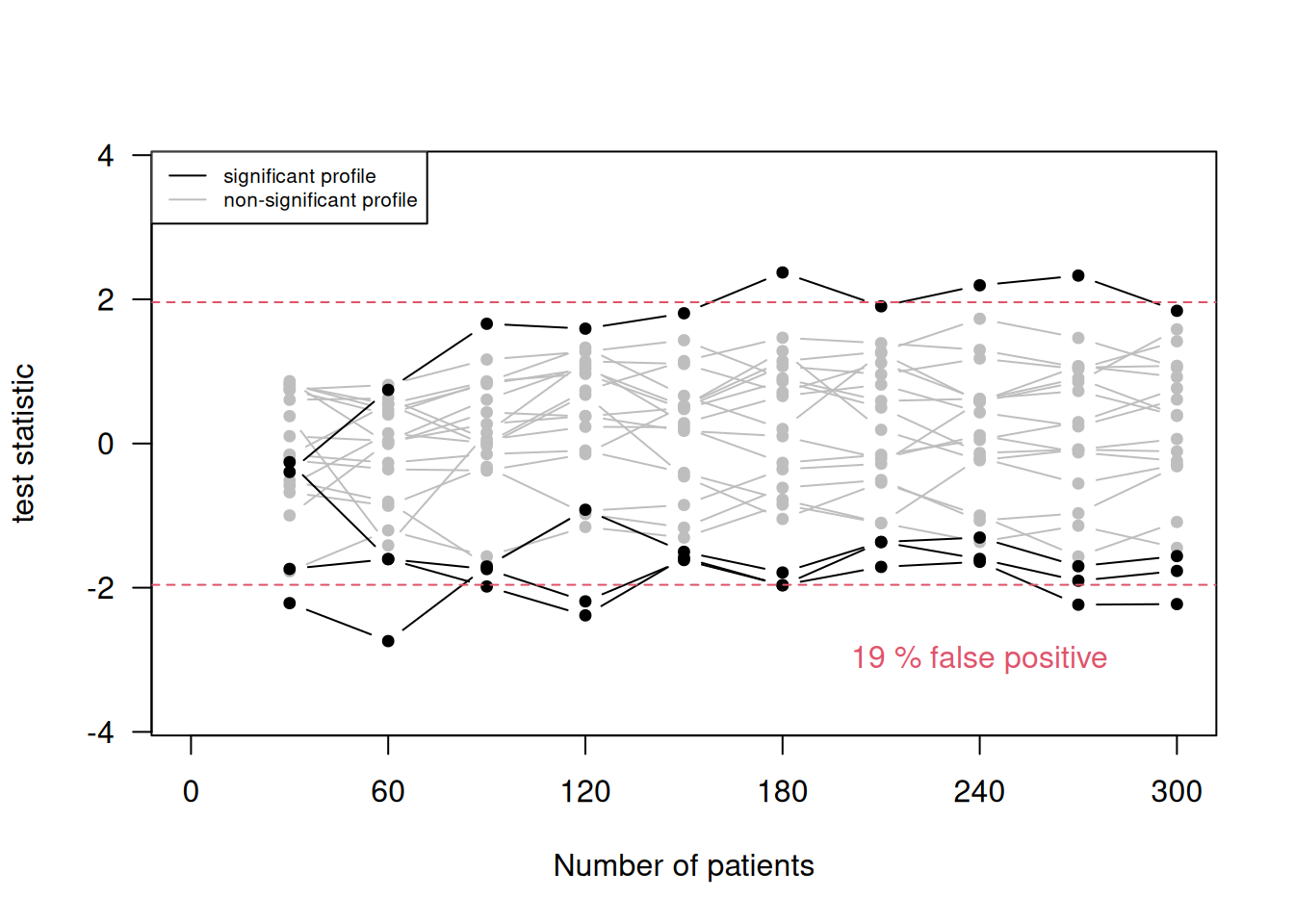
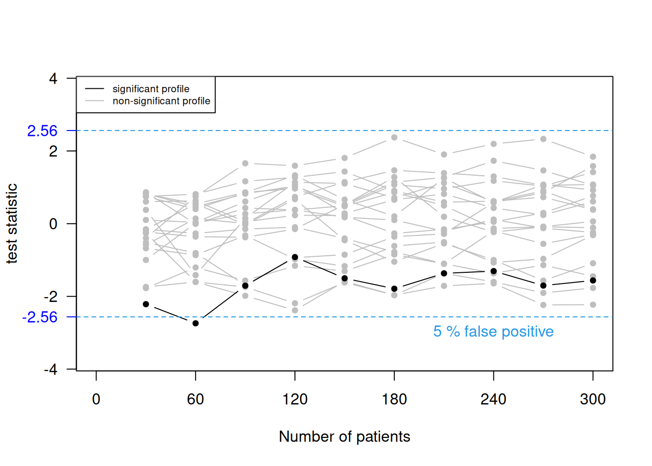
Figure 11.1: 20 selected profiles of the test statistic values based on the accumulating data and the false positive rate based on all 10000 simulations, once with the standard significance threshold (top) and once with an adjusted significance threshold (bottom).
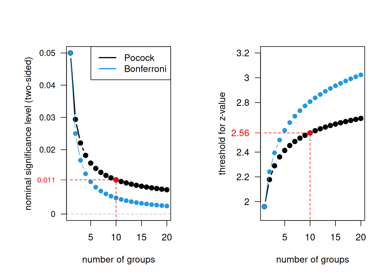
Figure 11.2: Pocock stopping rule and Bonferroni correction as a function of the number of groups.
The maximum total sample size T depends on the power to detect the clinically relevant difference and the maximum number of analyses N. In order to maintain a given power, the maximum total sample size T increases with increasing N. However, for \(N> 1\), there is always a chance that less than T patients will be needed.
Example 11.2 Consider a continuous outcome and fix \(\alpha=0.05\). Suppose that the goal is to detect a treatment difference of 0.5 standard deviation with power 90%. The maximal number \(N\) of analyses after every successive group of \(2n\) patients affects the nominal significance level \(\tilde \alpha\) and the maximum total sample size \(T = 2nN\), see Table 11.1.
| \(N\) | \(\tilde\alpha\) | \(n\) | \(T\) |
|---|---|---|---|
| 1 | 0.0500 | 84 | 168 |
| 2 | 0.0294 | 46 | 184 |
| 5 | 0.0158 | 20 | 200 |
| 10 | 0.0106 | 11 | 220 |
Other stopping rules
The Pocock stopping rule, where each test uses the same nominal significance level \(\tilde \alpha\), has two disadvantages. First, it is not too difficult for a trial to be halted early, which is considered as undesirable and uncompelling by some authors. Second, suppose that the trial terminates at the final analysis with \(\tilde \alpha < p < \alpha\). Many clinicians find it difficult to accept that the result of this trial is non-significant.
It is better to use a stopping rule \(a_1, a_2, \ldots, a_N\) where \(a_j\) is the significance threshold at the \(j\)-th interim analysis with \(a_1\) very small and \(a_j\) gradually increasing to \(a_N\) close to \(\alpha\). Three such stopping rules are shown in Table 11.2 and Figure 11.3. They all control the overall Type I error rate \(\alpha=5\%\) with \(N=5\) maximal interim analyses, except for the Haybittle-Peto approach which controls it only approximately.
| Method | 1 | 2 | 3 | 4 | 5 |
|---|---|---|---|---|---|
| Haybittle-Peto (1971) | 0.001 | 0.001 | 0.001 | 0.001 | 0.05 |
| Pocock (1977) | 0.0158 | 0.0158 | 0.0158 | 0.0158 | 0.0158 |
| O’Brien-Fleming (1979) | 5e-6 | 0.0013 | 0.0085 | 0.0228 | 0.0417 |
| Fleming et al. (1984) | 0.0038 | 0.0048 | 0.0053 | 0.0064 | 0.0432 |
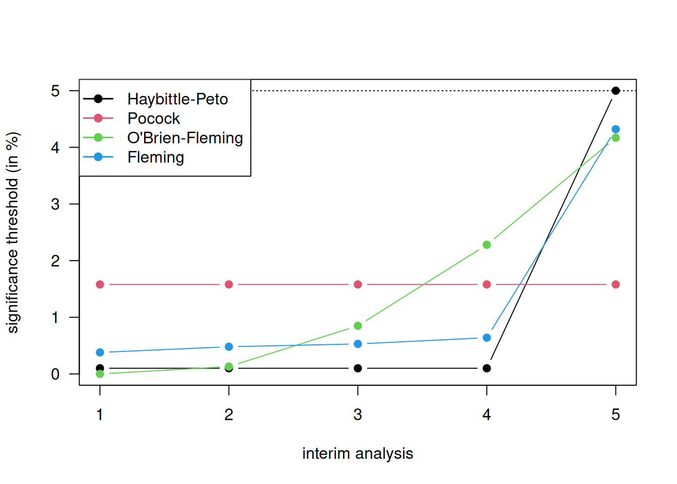
Figure 11.3: Different methods for stopping rules with \(5\) maximal interim analyses.
These stopping rules are implemented in the R package gsDesign.
The argument alpha is the one-sided significance level,
and the argument test.type is usually set to 1 (one-sided), i.e.,
we have no interest in stopping early for futility (lower bound).
Here we only use gsDesignfor relatively simple designs,
but many more things are possible. An alternative is the R package
rpact.
library(gsDesign)

## Pocock stopping rule
gsDesign(k = 3, alpha=0.025,
         sfu = "Pocock", test.type = 1)
## One-sided group sequential design with
## 90 % power and 2.5 % Type I Error.
## Sample
## Size
## Analysis Ratio* Z Nominal p Spend
## 1 0.384 2.29 0.011 0.0110
## 2 0.767 2.29 0.011 0.0079
## 3 1.151 2.29 0.011 0.0060
## Total 0.0250
##
## ++ alpha spending:
## Pocock boundary.
## * Sample size ratio compared to fixed design with no interim
##
## Boundary crossing probabilities and expected sample size
## assume any cross stops the trial
##
## Upper boundary (power or Type I Error)
## Analysis
## Theta 1 2 3 Total E{N}
## 0.0000 0.011 0.0079 0.0060 0.025 1.1391
## 3.2415 0.389 0.3421 0.1689 0.900 0.7210## One-sided group sequential design with
## 90 % power and 2.5 % Type I Error.
## Sample
## Size
## Analysis Ratio* Z Nominal p Spend
## 1 0.339 3.47 0.0003 0.0003
## 2 0.677 2.45 0.0071 0.0069
## 3 1.016 2.00 0.0225 0.0178
## Total 0.0250
##
## ++ alpha spending:
## O'Brien-Fleming boundary.
## * Sample size ratio compared to fixed design with no interim
##
## Boundary crossing probabilities and expected sample size
## assume any cross stops the trial
##
## Upper boundary (power or Type I Error)
## Analysis
## Theta 1 2 3 Total E{N}
## 0.0000 0.0003 0.0069 0.0178 0.025 1.0136
## 3.2415 0.0565 0.5288 0.3147 0.900 0.7987There are also other forms of stopping rules. A more flexible approach is based on the Lan-DeMets alpha spending function and does not require the maximum number of interim analyses to be specified in advance. Another popular approach to analyze accumulating data is Whitehead’s triangular test based on the score statistic \(Z\) and the Fisher information \(V\).
11.1.3 Problems of stopping at interim
If a trial terminates early, then there are problems with obtaining unbiased treatment effects due to the sequential nature of the trial. If a traditional analysis is performed in a trial that stops at interim because treatment is found to be significantly better than control, then the treatment effect estimate will be too large, the CI will be too narrow, and the \(P\)-value will be too small. Advanced methods for attempting to correct this bias are available, but rarely used, see Robertson et al (2023) and Robertson et al (2024) for recent reviews.
Example 11.3 We illustrate the problems of stopping at interim in a simulation example. Suppose that we have two equally sized treatment arms and a continuous primary outcome. The difference in means \(\theta\) is used as effect size. We fix the following analysis parameters: \(N=10\) interim analyses with Pocock bound \(z_P=2.56\) (nominal significance level \(\tilde \alpha = 0.011\)) and \(n=15\) patients per group and treatment arm to achieve a power of 75% to detect the true treatment effect \(\theta=0.35\) with standard deviation \(\sigma=1\). Significance at the \(k\)-th interim analysis implies the following minimum detectable difference (MDD, Compare Table 5.2) for the treatment effect estimate: \[\begin{equation*} \hat \theta \geq z_P \sqrt{2/(k \cdot n)}. \end{equation*}\]
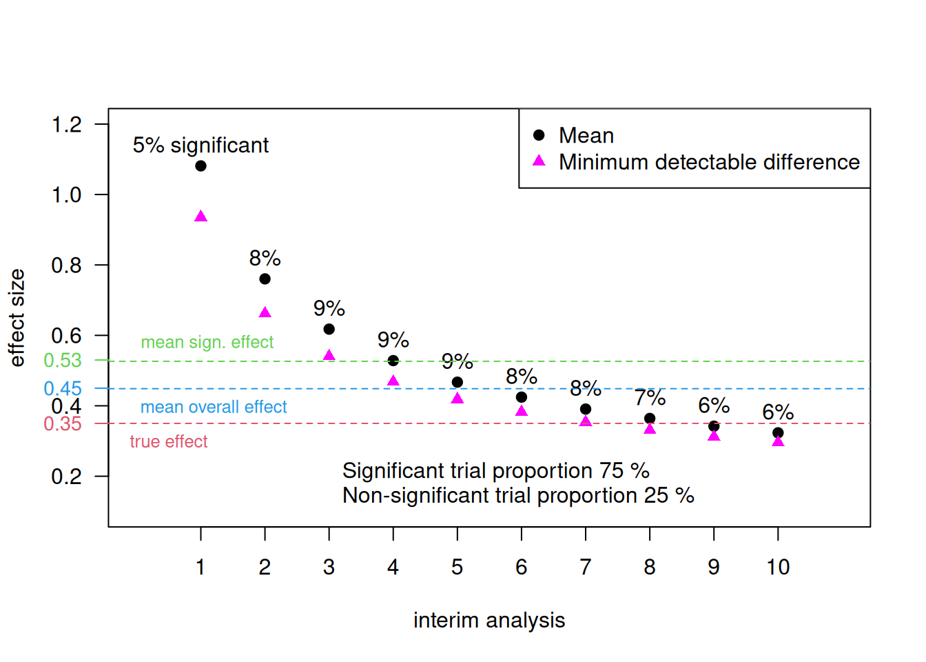
Figure 11.4: Effect sizes in a simulation with the Pocock stopping rule for a maximal number of 10 interim analyses (Example 11.3).
The effect size and minimum detectable difference for each interim analysis are displayed in Figure 11.4. The mean effect size of all significant trials is \(0.53 > 0.35\), the mean effect size of all non-significant trials is \(0.23 < 0.35\), and the mean effect size of all trials is \(0.45 > 0.35\).
11.2 The trial protocol
The trial protocol serves at least three purposes. First, it outlines the reasons for running a trial. Second, it is an operations manual for the trial, e.g.: assessment for eligibility, treatment allocation, blinding procedure, etc. Finally, it is the scientific design document for the trial, e.g.: methods for allocation, ways of assessing outcomes etc. The trial protocol needs approval by ethics committees, funding bodies, regulatory authorities etc. A statistical analysis plan (SAP) complements a trial protocol with more details on the methods planned to analyse the trial data. See Gamble et al (2017) and Stevens et al (2023) for guidelines and templates, respectively, for statistical analysis plans (SAPs).
Designing and reporting trials
A convincing report can only result from a convincing study design. Potential problems should be addressed already in the trial protocol to ensure that choices have not been influenced by the results. These can be for example problems of multiplicity such as which subgroups should be examined, which outcomes are primary and which are secondary, whether outcomes should be compared using baseline information, or whether the outcome variable should be transformed. Note that the most important statistical aspects need to be defined already in the study protocol (see Section 6.4.1).
Protocol deviations
Not all patients may adhere to the protocol, e.g. some may not take the medication in the quantities and at the times specified in the protocol, some may not turn up to the clinic for outcome measurements to be assessed, some may assert their right to withdraw from the study. In addition, ineligible patients may enter the trials, and other treatment than the one allocated may be administered.
Matthews (2006) (Section 10.2) gives examples of protocol deviations. They can be dealt with differently in the analysis:
Definition 11.1
- The per-protocol analysis compares groups of patients who were actually treated as specified in the protocol, excluding non-compliant patients.
- The as-treated analysis compares groups of patients as they were actually treated. No patients are excluded from this analysis.
- The intention-to-treat (ITT) analysis compares groups of patients as they were allocated to treatment.
The ITT principle states: “Compare the groups as if they were formed by randomization, regardless of what has happened subsequently to the patients” (Matthews, 2006, sec. 10.3). Any other way of grouping the patients cannot guarantee balance at the start of the treatment. Per-protocol or as-treated analyses are subject to possible confounding, so should be interpreted cautiously. On the other hand, analysis by the ITT principle may lead to attenuated treatment effects.
Example 11.4 The Angina Trial is an RCT comparing surgical versus medical treatment for angina. Primary outcome is 2-year mortality. In this trial, not all patients received the treatment they were allocated to.
##   Allocated Received No.Death No.Total No.Survived MortRate
## 1   Surgery  Surgery       15      369         354     4.07
## 2   Surgery Medicine        6       26          20    23.08
## 3  Medicine  Surgery        2       48          46     4.17
## 4  Medicine Medicine       27      323         296     8.36
This trial can be analyzed based on the three different analysis types. For the per-protocol analysis, we need to restrict the patients that we analyze.
## patients included in a per-protocol analysis
angina.perProtocol <- angina[Allocated==Received,]
print(angina.perProtocol)
## Allocated Received No.Death No.Total No.Survived MortRate
## 1 Surgery Surgery 15 369 354 4.07
## 4 Medicine Medicine 27 323 296 8.36## intention-to-treat analysis
tab.intentionToTreat <- xtabs(cbind(No.Death, No.Survived) ~ Allocated,
data=angina)
twoby2(tab.intentionToTreat)## 2 by 2 table analysis:
## ------------------------------------------------------
## Outcome : No.Death
## Comparing : Surgery vs. Medicine
##
## No.Death No.Survived P(No.Death) 95% conf.
## Surgery 21 374 0.0532 0.0349
## Medicine 29 342 0.0782 0.0549
## interval
## Surgery 0.0802
## Medicine 0.1102
##
## 95% conf. interval
## Relative Risk: 0.6801 0.3950 1.1711
## Sample Odds Ratio: 0.6622 0.3706 1.1832
## Conditional MLE Odds Ratio: 0.6625 0.3519 1.2284
## Probability difference: -0.0250 -0.0616 0.0104
##
## Exact P-value: 0.1882
## Asymptotic P-value: 0.1639
## ------------------------------------------------------## per-protocol analysis
tab.perProtocol <- xtabs(cbind(No.Death, No.Survived) ~ Allocated,
data=angina.perProtocol)
twoby2(tab.perProtocol)## 2 by 2 table analysis:
## ------------------------------------------------------
## Outcome : No.Death
## Comparing : Surgery vs. Medicine
##
## No.Death No.Survived P(No.Death) 95% conf.
## Surgery 15 354 0.0407 0.0247
## Medicine 27 296 0.0836 0.0579
## interval
## Surgery 0.0663
## Medicine 0.1192
##
## 95% conf. interval
## Relative Risk: 0.4863 0.2634 0.8979
## Sample Odds Ratio: 0.4645 0.2426 0.8896
## Conditional MLE Odds Ratio: 0.4650 0.2254 0.9256
## Probability difference: -0.0429 -0.0816 -0.0070
##
## Exact P-value: 0.0246
## Asymptotic P-value: 0.0207
## ------------------------------------------------------## as-treated analysis
tab.asTreated <- xtabs(cbind(No.Death, No.Survived) ~ Received,
data=angina)
twoby2(tab.asTreated)## 2 by 2 table analysis:
## ------------------------------------------------------
## Outcome : No.Death
## Comparing : Surgery vs. Medicine
##
## No.Death No.Survived P(No.Death) 95% conf.
## Surgery 17 400 0.0408 0.0255
## Medicine 33 316 0.0946 0.0680
## interval
## Surgery 0.0646
## Medicine 0.1300
##
## 95% conf. interval
## Relative Risk: 0.4311 0.2444 0.7605
## Sample Odds Ratio: 0.4070 0.2226 0.7441
## Conditional MLE Odds Ratio: 0.4074 0.2088 0.7689
## Probability difference: -0.0538 -0.0922 -0.0184
##
## Exact P-value: 0.0031
## Asymptotic P-value: 0.0035
## ------------------------------------------------------11.3 Additional references
More information about RSTs and sequential methods can be found in Bland (2015) (Ch. 9.11) and in Todd et al (2001), about ITT in Bland (2015) (Ch. 2.6), about monitoring accumulating data in Matthews (2006) (Ch. 8) and about protocols and protocol deviations in Matthews (2006) (Ch. 10). Studies where the methods from this chapter are used in practice are for example ACRE Trial Collaborators and others (2009), Durán-Cantolla et al (2010), Burgess et al (2005)