Chapter 15 Fitting Nonlinear Data With OLS

This chapter has not yet been updated for the Spring 2021 offering of HE-802. It is not yet ready for student use in Spring 2021 and will likely be updated before it is assigned to students in the course calendar.

Now that we have covered the most important type of linear regression analysis, we can start to explore different ways in which regresson analysis can be used. As you do data analysis of your own, you will very frequently find that your data and/or your regression results violate some of the stipulated assumptions of OLS linear and logistic regression models.

This week, we will go through an example together about how to improve the fit of a linear regression model by specifying it differently, such that we can fit a regression curve to non-linear data. In this process, you will see an example of how OLS regression assumptions are violated and then fixed.

In your assignment this week, you will practice the same procedure that is demonstrated in the chapter. You will fit non-linear data using OLS linear regression and overcome a violation of the OLS regression assumptions.

This week, our goals are to…

Identify situations in which OLS regression assumptions are violated.
Practice transforming independent variables and including them in regression models, to explore non-linear relationships between independent and dependent variables, without violating OLS regression assumptions.

15.1 Quadratic (Squared) Relationships

15.1.1 Non-linear Data

Before this week, we have learned how to fit linear relationships in our data. These models required the assumption that the independent variables varied linearly with the dependent variable.

But what if our data does not vary linearly with our dependent variable? This section will introduce you to one transformation you can apply to your data to use regression models to discover and fit non-linear relationships between your variables.

The most important non-linear relationship that I would like us to look at is what is called a quadratic relationship. Below, we will go through an example that shows an attempt to fit data using a linear model only and then how a non-linear, quadratic model can actually help us fit our data and uncover a trend better.

15.1.2 Linear Model With Non-Linear Data

To begin our example, consider the following data called mf (which stands for “more fitness”), which is a modification of the fitness data that we looked at before. Here are the variables in this data:

lift – How much weight each person lifted. This is the dependent variable, the outcome we are interested in.
hours – How many hours per week each person spends weightlifting. This is the independent variable we are interested in.

Our question is: What is the association between lift and hours?

First, we’ll load the data into R. You can copy and paste this and run it too!

name <- c("Person 01", "Person 02", "Person 03", "Person 04", "Person 05", "Person 06", "Person 07", "Person 08", "Person 09", "Person 10", "Person 11", "Person 12", "Person 13", "Person 14", "Person 15", "Person 16", "Person 17", "Person 18", "Person 19", "Person 20", "Person 21", "Person 22", "Person 23", "Person 24", "Person 25", "Person 26", "Person 27", "Person 28", "Person 29", "Person 30")
hours <- c(1,2,3,4,5,6,7,8,9,10,1,2,3,4,5,6,7,8,9,10,1,2,3,4,5,6,7,8,9,10)
lift <- c(5,15,20,30,37,48,50,51,51,51,6.9,19.5,29.5,40.4,45.0,48.0,50.9,50.3,51.4,51.8,9.3,19.1,29.5,40.0,44.2,47.2,50.6,51.7,51.6,50.2)

mf <- data.frame(name, lift, hours)
mf

##         name lift hours
## 1  Person 01  5.0     1
## 2  Person 02 15.0     2
## 3  Person 03 20.0     3
## 4  Person 04 30.0     4
## 5  Person 05 37.0     5
## 6  Person 06 48.0     6
## 7  Person 07 50.0     7
## 8  Person 08 51.0     8
## 9  Person 09 51.0     9
## 10 Person 10 51.0    10
## 11 Person 11  6.9     1
## 12 Person 12 19.5     2
## 13 Person 13 29.5     3
## 14 Person 14 40.4     4
## 15 Person 15 45.0     5
## 16 Person 16 48.0     6
## 17 Person 17 50.9     7
## 18 Person 18 50.3     8
## 19 Person 19 51.4     9
## 20 Person 20 51.8    10
## 21 Person 21  9.3     1
## 22 Person 22 19.1     2
## 23 Person 23 29.5     3
## 24 Person 24 40.0     4
## 25 Person 25 44.2     5
## 26 Person 26 47.2     6
## 27 Person 27 50.6     7
## 28 Person 28 51.7     8
## 29 Person 29 51.6     9
## 30 Person 30 50.2    10

Now, we’ll fit the data following our first instinct, OLS linear regression:

summary(reg1 <- lm(lift ~ hours, data = mf))

## 
## Call:
## lm(formula = lift ~ hours, data = mf)
## 
## Residuals:
##      Min       1Q   Median       3Q      Max 
## -11.3582  -5.5729   0.3623   5.3844   9.5006 
## 
## Coefficients:
##             Estimate Std. Error t value Pr(>|t|)    
## (Intercept)  11.5111     2.6109   4.409 0.000139 ***
## hours         4.8471     0.4208  11.519 3.88e-12 ***
## ---
## Signif. codes:  0 '***' 0.001 '**' 0.01 '*' 0.05 '.' 0.1 ' ' 1
## 
## Residual standard error: 6.62 on 28 degrees of freedom
## Multiple R-squared:  0.8258, Adjusted R-squared:  0.8195 
## F-statistic: 132.7 on 1 and 28 DF,  p-value: 3.884e-12

As we expected, lifting weights weekly is associated with increased ability to lift weight. The $R^2$ statistic is very high, meaning the model fits quite well. So far, everything seems fine. Now let’s let’s look at diagnostic plots:

library(car)
residualPlots(reg1)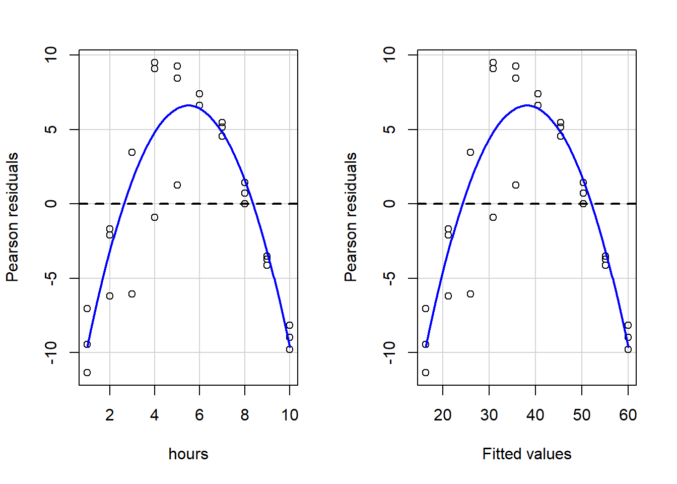

##            Test stat Pr(>|Test stat|)    
## hours        -11.466        6.988e-12 ***
## Tukey test   -11.466        < 2.2e-16 ***
## ---
## Signif. codes:  0 '***' 0.001 '**' 0.01 '*' 0.05 '.' 0.1 ' ' 1

When we visually inspect these plots, we see that the blue lines are not even close to straight, so key OLS assumptions are violated. And if we look at the written output, it is clear that we fail both a) the goodness of fit test for hours, the only independent variable, and b) the Tukey test for the overall model.

Clearly, we need to re-specify our regression model so that we can fit the data better and also so that we can avoid violating OLS regression assumptions. Keep reading to see how we can do that!

15.1.3 Inspecting The Data

Just now, we saw that running a linear regression the way we normally do does not fit our data well. But we don’t necessarily know how to fix the problem. A good first step is to visually inspect the relationship that we are trying to understand.

Let’s look at a scatterplot of the data to see what might be going on. Below is a plot with lift—our dependent variable of interest—and hours—our independent variable of interest—plotted against each other.

plot(mf$hours, mf$lift)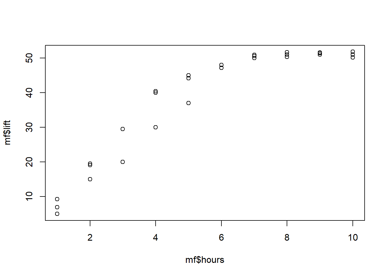

The data are not really in a straight line. It starts off sort of linear (looking from lower to higher number of hours), but then seems to level off. Clearly, this is a non-linear trend, meaning that lift and hours do not vary linearly with one another. A straight line is not the best description of their relationship.

But linear regression only fits linear trends. We have to somehow tell the computer that it is free to fit a non-linear, or curvilinear trend to the data. To do this, we add a quadratic term as an independent variable in the model. A quadratic term just means a squared term.

As you may recall from math classes before, a polynomial equation that has an $x^2$ term in it (and no $x$ terms with higher exponents—such as $x^3$), such as $y = x^2$, will result in a parabola.

So our new goal is to fit not a line, but a parabola to our data.

Read on to see how to do this in R and how to interpret the results!

15.1.4 Preparing The Data

To tell R that we want to fit a parabola rather than a line to our data, we will need to add a squared regression term to our regression formula in the lm() command. First, we need to create a squared version of the independent variable that we want to add to the model. In this case, that variable is hours.

Note that in the future you will likely have regression models with more than one independent variable. In that situation, you can add squared terms for some but not all of the independent variables into the model. (You can also add squared terms for all of the variables if you want). You do not need to add squared terms for all independent variables, only the ones that you suspect have a curvilinear/parabolic relationship with the dependent variable.

Here’s how we create the squared term:

mf$hoursSq <- mf$hours^2

The code above is saying the following:

mf$hoursSq – Within the dataset mf, create a new variable called hoursSq.
<- – The new variable to left will be assigned to the value generated by the code to the right.
mf$hours^2 – Within the dataset mf, get the variable hours and square it.

Now, let’s inspect the data once again:

mf

##         name lift hours hoursSq
## 1  Person 01  5.0     1       1
## 2  Person 02 15.0     2       4
## 3  Person 03 20.0     3       9
## 4  Person 04 30.0     4      16
## 5  Person 05 37.0     5      25
## 6  Person 06 48.0     6      36
## 7  Person 07 50.0     7      49
## 8  Person 08 51.0     8      64
## 9  Person 09 51.0     9      81
## 10 Person 10 51.0    10     100
## 11 Person 11  6.9     1       1
## 12 Person 12 19.5     2       4
## 13 Person 13 29.5     3       9
## 14 Person 14 40.4     4      16
## 15 Person 15 45.0     5      25
## 16 Person 16 48.0     6      36
## 17 Person 17 50.9     7      49
## 18 Person 18 50.3     8      64
## 19 Person 19 51.4     9      81
## 20 Person 20 51.8    10     100
## 21 Person 21  9.3     1       1
## 22 Person 22 19.1     2       4
## 23 Person 23 29.5     3       9
## 24 Person 24 40.0     4      16
## 25 Person 25 44.2     5      25
## 26 Person 26 47.2     6      36
## 27 Person 27 50.6     7      49
## 28 Person 28 51.7     8      64
## 29 Person 29 51.6     9      81
## 30 Person 30 50.2    10     100

You can see that a new column of data has been added for the new squared version of the independent variable hours. Keep in mind that R automatically squared the value of hours separately for us in each row and then placed that new squared value in that same row in the new column for hoursSq. For example, see row #4. This person, labeled as Person 4, spends 4 hours lifting weights per week, which we can see in row #4 in the hours column. And then we can see that the computer has added the number 16 in the column hoursSq for Person 4.

Now that we have our new squared variable in the model, we can do another regression.

15.1.5 Running and Interpreting Quadratic Regression

We are now ready to run our new regression with a quadratic (squared) term included as an independent variable. To do this, we use the same lm() command that we always do, but we include our newly created squared term—hoursSq—as an independent variable. It is important to note that even though we are now adding the hoursSq variable to our model, we still need to keep the un-squared hours variable in as well.

Here is the code to run the new regression:

summary(reg2 <- lm(lift ~  hours + hoursSq, data = mf))

## 
## Call:
## lm(formula = lift ~ hours + hoursSq, data = mf)
## 
## Residuals:
##     Min      1Q  Median      3Q     Max 
## -7.6556 -0.8003  0.2714  1.4855  4.6908 
## 
## Coefficients:
##             Estimate Std. Error t value Pr(>|t|)    
## (Intercept) -6.12500    1.88959  -3.241  0.00315 ** 
## hours       13.66513    0.78917  17.316 3.80e-16 ***
## hoursSq     -0.80164    0.06992 -11.466 6.99e-12 ***
## ---
## Signif. codes:  0 '***' 0.001 '**' 0.01 '*' 0.05 '.' 0.1 ' ' 1
## 
## Residual standard error: 2.783 on 27 degrees of freedom
## Multiple R-squared:  0.9703, Adjusted R-squared:  0.9681 
## F-statistic: 441.2 on 2 and 27 DF,  p-value: < 2.2e-16

One of the first numbers that should pop out at you is the extremely high $R^2$ statistic. This indicates that the new regression model fits the data extremely well.¹⁷⁰ The variation in the independent variables explains over 90% of the variation in the dependent variable!

Keep in mind that we did not add any new data to the model. All we did is tell the computer to look for a curved, parabolic trend, rather than solely a linear trend. Doing this allowed us to create a regression model that fit our data much better than before.

The equation for this new quadratic regression result is:

\[\hat{lift} = -6.13 + 13.67*hours -0.8*hours^2\]

If we rewrite this in terms of just Y and X, it looks like this:

\[\hat{y} = -6.13 + 13.67x -0.8x^2\]

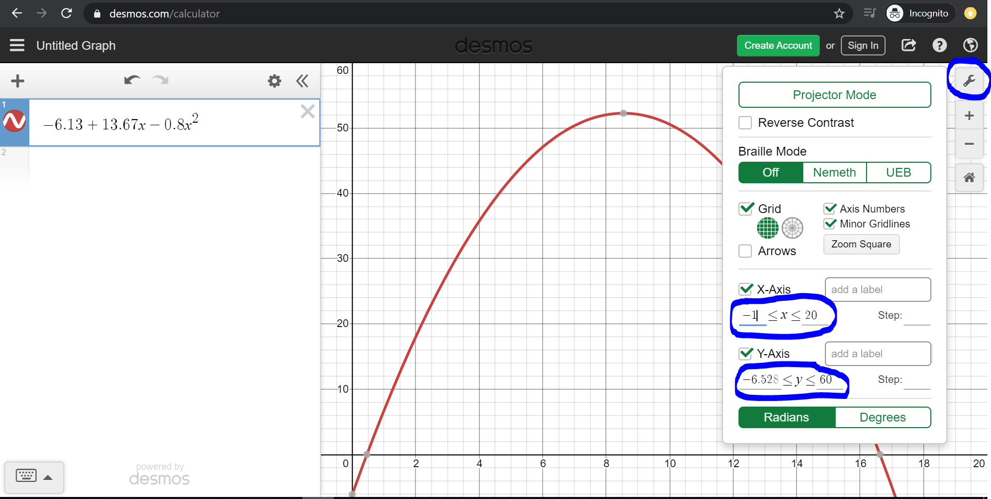
This is the equation of the parabola that fits our data. Let’s plot this equation into a graphing calculator. Click here to open a graphing calculator. Copy and paste the following into the graphing calculator:

-6.13 + 13.67x -0.8x^2

Next, change the axes by clicking on the wrench in the top-right corner, so that the parabola is framed well.

Please follow these steps and see the screenshot below:

Paste -6.13 + 13.67x -0.8x^2 into the equation box in the top-left corner.
Click on the wrench in the top-right corner which is circled in blue.
Change the x-axis to range from approximately -1 to 20 in the bottom right, where the blue circle is.
Change the y-axis to range from approximately -5 to 60 in the bottom right, where the blue circle is.

Then you should see the entire portion of the parabola that is in the range of our data.

We can also plot this in R, along with our data points:

eq2 = function(x){-6.13 + 13.67*x -0.8*(x^2)}

ggplot(data.frame(x=c(1, 14)), aes(x=x)) + stat_function(fun=eq2) + geom_point(aes(x=hours, y=lift), data = mf)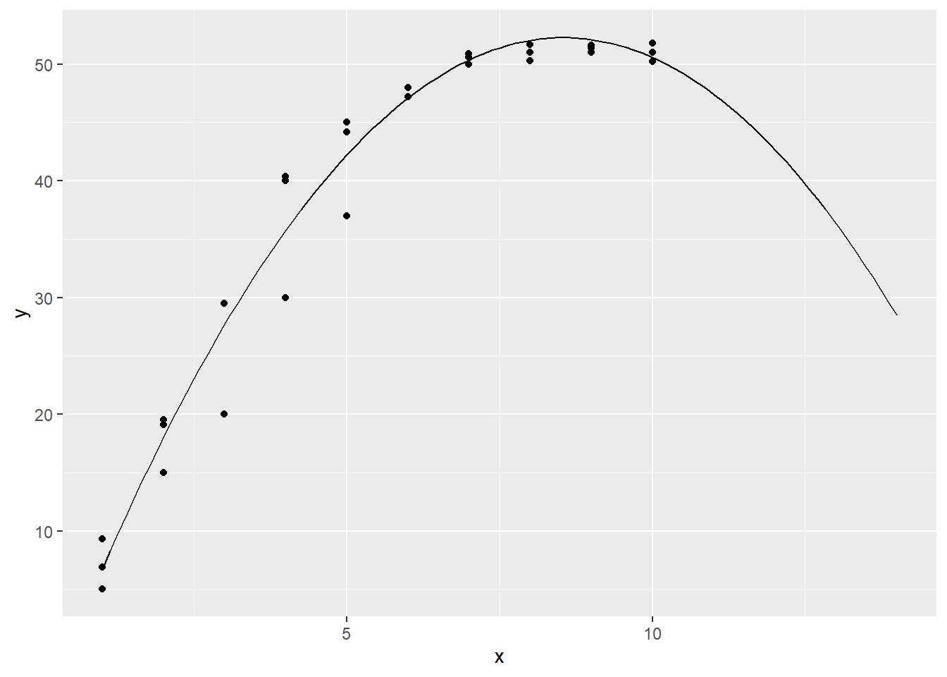

Our new model seems to fit the data pretty well, and it captures the nonlinear nature of the relationship between lift and hours.

This result tells us that weight lifting capability increases as weekly weightlifting hours go up, until we reach about 7 hours per week of weightlifting. The slope is steep at first (at lower levels of hours on the x-axis) but then it levels off and becomes less steep. This is basically suggesting that the gains or returns to weightlifting level off as you train more.

Such a trend is sometimes referred to as decreasing/diminishing marginal returns. The slope becomes less and less positive at higher values of the independent variable. In other words, the added benefit of each additional hour of weightlifting is predicted to be less and less as you weightlift more.

For people who do more than about 10 hours per week, the model is actually predicting a decrease in weightlifting capability with each increased hour of weight training. This prediction is probably incorrect. So we have to remember that even though this model fits our data much better, it also makes predictions that might not always make sense when we look at the extreme ends of our data range.

Note that we left the unsquared hours variable in the model, in addition to the hoursSq variable. It is essential to leave the unsquared variable in the model as well. Do not remove it! Also note that this is still OLS linear regression, even though we used it to fit a non-linear trend.

15.1.6 Residual Plots For Quadratic Regression

Above, we ran a quadratic regression and it appears that we were able to fit our regression model to the data quite well. But the very next thing we should always do is to look at the residual plots of the new regression model.

Here they are:

residualPlots(reg2)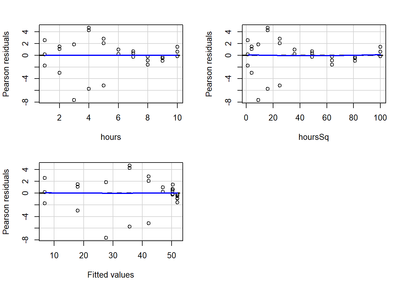

##            Test stat Pr(>|Test stat|)   
## hours         2.9829         0.006135 **
## hoursSq       0.2386         0.813257   
## Tukey test    0.0515         0.958897   
## ---
## Signif. codes:  0 '***' 0.001 '**' 0.01 '*' 0.05 '.' 0.1 ' ' 1

As you’ll recall from earlier in the chapter, when we did not have a squared term in the regression, our residuals appeared to be correlated with the independent variable hours as well as with the fitted values of the regression. You can scroll up and have another look. You will see very curved blue lines.

Now look again at the new residual plots above. They look much better and are no longer violating the tested regression assumptions! The blue lines are straight, horizontal, and hugging the 0-line in the charts.

Remember, in this example, above we only ran the residual plots diagnostics. However, when you use OLS linear regression for real research, instead of practice like this, you have to test all of the OLS regression assumptions, just like you did in a previous assignment. Before testing these assumptions, you cannot fully trust the results you see in the regression output summary!

Also, keep in mind that the mf data used in this example is fake data that was created to illustrate this method. But in your assignment for this week, you will use real data to examine a non-linear trend on your own, following the same procedure above.

15.1.7 Other Transformations – Optional

Reading this section is completely optional and not required. The squared/quadratic transformation that we examined in detail above is not the only way to transform your data. The quadratic transformation is only to fit a parabola to your data. If you notice that the relationship you want to study is non-linear but likely does not follow a parabolic trajectory, there are other transformations that you can try. We will not look at these other transformations much or at all in this course, but it is important to be aware that other options exist.

Log transformations are one of the most commonly used transformations to improve the fit of regression models to data.

Here are some resources related to log and other transformations:

Interpreting Log Transformations in a Linear Model
Chapter 14 “Transformations” in Applied Statistics with R.
Transformations of Variables – This resource features a nice table that compares many types of transformations to each other.

15.2 Assignment

In this week’s assignment, you will practice using OLS linear regression to fit a non-linear trend in data. You should follow a similar procedure to what was presented earlier in this chapter to fit nonlinear data. The purpose of this activity is to practice identifying and fitting non-linear relationships in R. You will be evaluated based on your ability to follow the example earlier in this chapter and fit the data in the dataset below.

To begin, run the following code to load the data:

if (!require(openintro)) install.packages('openintro')
library(openintro)

data(hsb2)
h <- hsb2

summary(h)

You should also run the command ?hsb2 in the console to read more about the dataset, which is called the High School and Beyond survey.¹⁷¹

For this assignment, use the following variables:

Dependent Variable: math
Independent Variables: ses, write

15.2.1 Visualize The Data

Task 1: Use the plot() command to plot this data. Make sure that the dependent variable appears on the vertical axis and the numeric independent variable appears on the horizontal axis.

15.2.2 Linear Regression

Task 2: Run an OLS linear regression to see if these two independent variables are linearly associated or not with the dependent variable (do not yet try to fit a non-linear trend). Call this regression mod1.

Task 3: Generate residual plots for mod1. Interpret both the visual results and the numeric outputs.

15.2.3 Quadratic Regression

Task 4: Add a squared term to the regression for the appropriate independent variable and run the regression. Call this mod2.

Task 5: Generate residual plots for mod1. Interpret both the visual results and the numeric outputs.

Task 6: Compare $R^2$ values for mod1 and mod2. Based on the residual plots results, are both models trustworthy? Or only one or neither?

Task 7: Write out and interpret the equation for mod2. Note that it may help to visualize the equation before you interpret it.

15.2.4 Visualize Results

Task 8: Put the equation into a graphing calculator. Click here to open a graphing calculator. Be sure to adjust the axes by clicking on the wrench in the top-right corner. You do not need to submit anything related to this task.

Task 9: Optional. This task is not required. Create a scatterplot using ggplot which plots math against write. The plot should show both the individual points as well as the predicted regression equation from mod2. Be sure to put the correct variable on the correct axis!

15.2.5 Logistical Tasks

Task 10: Please include any questions or feedback you have that you wrote down as you read the chapter and did the assignment this week.

Task 11: Please submit your assignment to the online dropbox in D2L as a PDF or HTML file, as usual.

In fact, when $R^2$ is so high with social science data, it can sometimes be a red flag that something is wrong. It may indicate that one of your independent variables is so similar to your dependent variable that it is not meaningful and/or useful to study the relationship between these two variables and the concepts that they measure.↩︎
The hsb2 data is part of the openintro package, which is why we loaded that package before using the data() command to load the data into R.↩︎