Chapter 3 Feb 1–7: R Practice
This chapter has now been updated for spring 2021 and is ready to be used during the week of February 1–7 2021.
This week, our goals are to…
Download and install R and RStudio on your own computer.
Become oriented to the basic use of R and RStudio.
Conduct basic exploratory data analysis in R and RStudio.
Announcements and reminders
In this week’s chapter, there is an orientation to R and RStudio. Please follow along with this orientation on your own computer. A series of videos will walk you through this process. You DO NOT have to submit these “Orientation Tasks” as part of the assignment you submit at the end of this week. You ONLY need to submit to us the tasks in the assignment section in this chapter.
Once you have completed the Orientation section, I recommend that you pause and look at this week’s assignment. You can begin the assignment right away and refer to the chapter for how to do each step in the assignment. Most parts of the assignment require you to take code demonstrated in the chapter and modify it to accomplish the tasks requested in the assignment. Note that there is more in the chapter than you need to know for the assignment. Some portions of the chapter can simply serve as a reference to you for the future as you do more complex analysis later in the course. Feel free to ask Anshul and Nicole for suggestions on how to streamline this process so that it is efficient.
Please continue to contact Anshul and Nicole with with any questions you might have as you go through this week’s work. It would also be great if you let us know about any ambiguity in the content or instructions. We can also set up Zoom meetings on any day you would like to answer any questions you might have and support you as you go through this week’s content and do the assignment. Please do not hesitate to request a meeting. Learning statistics is a very social process.
3.1 Orientation to R and RStudio
So far in our time together, we have used tools such as spreadsheets and online tools to analyze data. Starting this week and for the majority of the rest of the course, we will do all of our quantitative methods work within a single data analysis platform. This week, we will install and practice using the computer software that will make this possible. We will be using a programming language called R, which is a programming language designed for data analysis and similar tasks. We will use the programming language R within a computer software called RStudio. R is kind of like English; it is the language you will be using to do data analysis. RStudio is kind of like Microsoft Word; it is one software that facilitates your use of the language R.
3.1.1 Basic use
We’ll start with some basics to get you set up and navigate within R and RStudio. Below, there is a list of “Orientation Tasks” for you to complete. You DO NOT have to submit these tasks as part of this week’s assignment. You should just do the Orientation Tasks below on your own to make sure they work for you on your computer. You only need to submit to us instructors the tasks in the assignment below.
The following video will walk you through the first steps of installing and using R and RStudio.
The video above can be viewed externally at https://youtu.be/_FVq-Vyyyfs.
Orientation Task 1: Download and install the appropriate version of R from https://cran.r-project.org/mirrors.html. Choose any link in your country or a nearby country.
Orientation Task 2: Download and install the appropriate version of RStudio from https://rstudio.com/products/rstudio/download/. Click on the Download button for the free version of RStudio Desktop.
Orientation Task 3: Create a new R file.
To create the new R file, click on File -> New File -> R Script.
You can think of an R file as a Microsoft Word file but for data analysis.
Orientation Task 4: Save the new R file you just created. You could also create a new folder for all your work in our class, if you want, and save your R file in there.
Orientation Task 5: Find your new file within the Files tab within RStudio.
Orientation Task 6: Type 2+3 into a line of your new R file and then click the Run button. Locate the console and see what happened there. It should look approximately like this:
2+3## [1] 5Orientation Task 7: In a new line of your R file, type 2*3 and click on Run. You should see something like this in the console:
2*3## [1] 6As you can see, R can help us do basic arithmetic. You could also type 2-3 or 2/3 for subtraction and division. And you can of course change the numbers 2 and 3 to other numbers.
3.1.2 Data loading and viewing
Now it’s time to load some data and look at it together in R and RStudio!
The following video will demonstrate this process.
The video above can be viewed externally at https://youtu.be/A9mQSqbx2hE.
Orientation Task 8: Let’s make a new dataset called d, using the code below.
Type this code into a new line of your R file and run it:
d<-mtcarsNow look in your Environment tab in RStudio. You should see a new data item called d.
What we did using the command above is that we created a new data object called d and we assigned d to contain the data within mtcars. mtcars is a dataset that comes along with R. It is built-in for us to practice with, like we are doing now!
Orientation Task 9: You can run the command ?mtcars to pull up some information about this data, if you would like.
Orientation Task 10: Type View(d) (with a capital V) into your R code file (in a new line, of course!) and run it.
A data viewer could pop up in a new tab, showing you your dataset in spreadsheet view.
Close the data viewer.
Orientation Task 11: Double click on d in the Environment tab. This should also bring up the data viewer.
Orientation Task 12: Now let’s inspect our data in the data viewer. What are some of your observations?
Orientation Task 13: What does each row in the data represent?
Orientation Task 14: What does each column in the data represent?
3.1.3 Descriptive statistics
Let’s go back to the R code file tab and do some simple analysis on our data. This is demonstrated in the video below.
The video above can be viewed externally at https://youtu.be/SNF01zoJ42I.
Orientation Task 15: Type d$ into your code file (in a new line, of course). A list of columns (variables) should pop up. Select mpg.
Now your line of code should say d$mpg.
Go ahead and run that line. You should get a result like this:
d$mpg## [1] 21.0 21.0 22.8 21.4 18.7 18.1 14.3 24.4 22.8 19.2 17.8 16.4 17.3 15.2 10.4
## [16] 10.4 14.7 32.4 30.4 33.9 21.5 15.5 15.2 13.3 19.2 27.3 26.0 30.4 15.8 19.7
## [31] 15.0 21.4Above, the computer gave you all of the data just from the column labeled mpg from our data.
Orientation Task 16: Now let’s calculate the mean of the column (variable) mpg.
mean(d$mpg)## [1] 20.09062Remember, put the command above into a new line of your code file and then run it. And you should see the result above in your console.
Orientation Task 17: How about the standard deviation of mpg? See below.
sd(d$mpg)## [1] 6.026948We have now calculated the mean and standard deviation of the mpg variable.
Orientation Task 18: We can also get a summary of the mpg variable as follows. Please add it to your code file and try it out!
summary(d$mpg)## Min. 1st Qu. Median Mean 3rd Qu. Max.
## 10.40 15.43 19.20 20.09 22.80 33.90The output above gives us a number of metrics, although it does not include standard deviation.
Orientation Task 19: Try running the mean, sd, and summary commands for a different variable that you choose.
3.1.4 Simple visualizations
We will continue with our brief exploration of our data by making some visualizations, as shown in this video:
The video above can be viewed externally at https://youtu.be/qS3Fh2S7Kd4.
Orientation Task 20: Run the command hist(d$mpg) (again, make sure you’re adding the command in a new line of your code file). You should get a histogram in your Viewer in RStudio.
hist(d$mpg)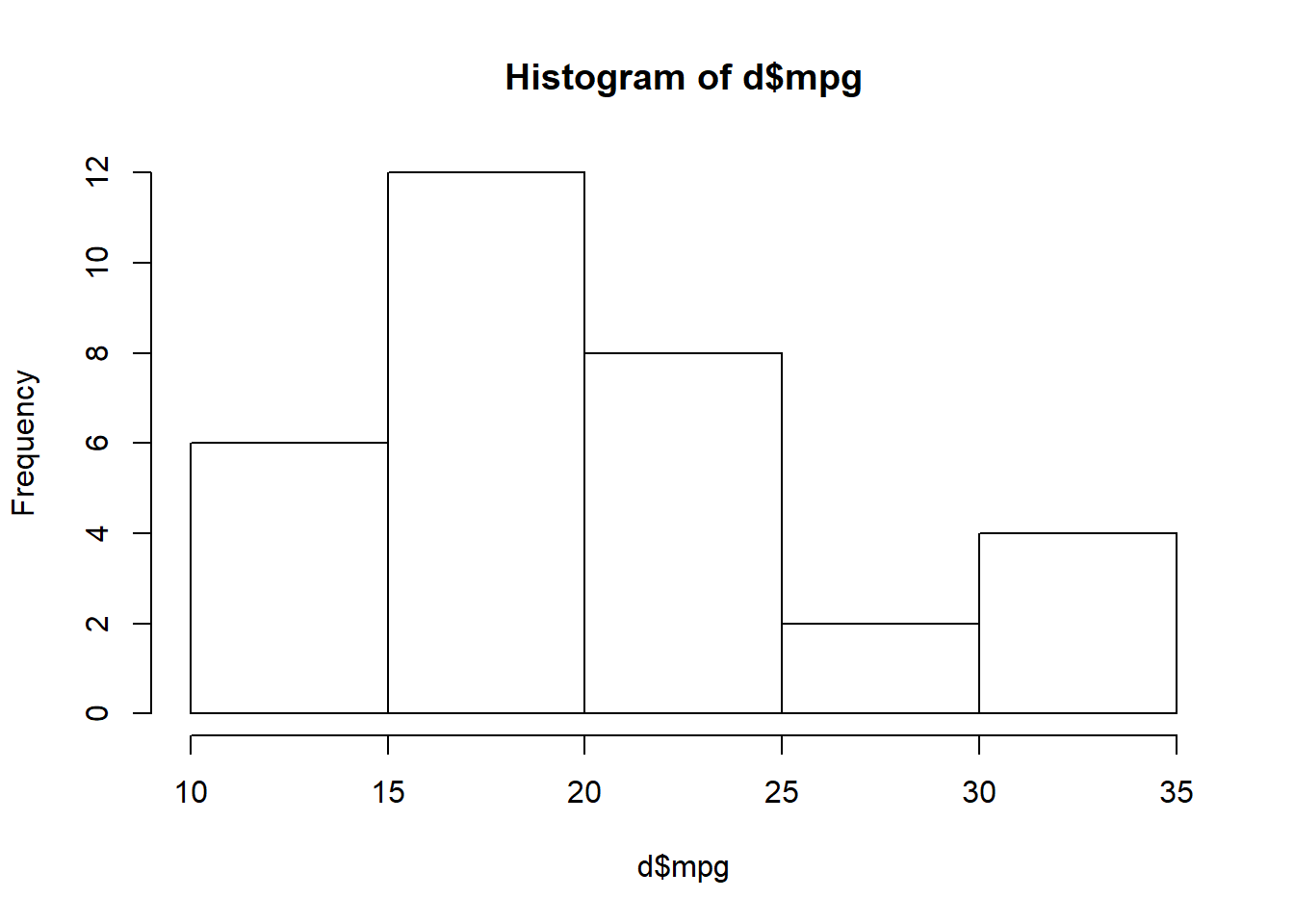
Orientation Task 21: And now let’s make a scatterplot using plot(d$wt,d$mpg).
plot(d$wt,d$mpg)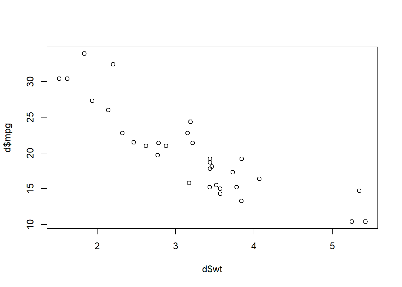
Above, we see that the more a car weighs (wt), the worse its fuel efficiency (mpg).
Orientation Task 22: Try making some other histograms and scatterplots!
3.1.5 Installing and loading packages
Finally, we will practice installing and loading packages to make sure this functionality is working correctly on your computer.
This video shows how to load a package:
The video above can be viewed externally at https://youtu.be/66HUNn4-92k.
As always, make sure that you put all new lines of code into your R code file.
Orientation Task 23: Run the command install.packages("car"). You should then see a bunch of output in the console. The process might take a while.
Once the process is over, the car package should be installed on your computer. You can see a list of installed packages in the Packages tab, if you want. There will be many packages there.
Orientation Task 24: Finally, run the command library(car) to load the car package into your current R session.
You have reached the end of the R and RStudio orientation process!
3.2 Loading and Exploring Data in R
In this section of the chapter, we will learn how to set R’s working directory, load data from an Excel file into R, make descriptive tables, subset our data, transform variables (columns in our data), recode variables, and remove duplicate observations (rows in our data). You will also practice skills such as installing and loading any required R packages, writing code into an R script file, and saving your work.
As you go through this section of this chapter, I recommend that you follow along by copying and pasting all of the provided code below into your own R file on your own computer.
3.2.1 Set the Working Directory in R and RStudio
As you practiced during our orientation procedure above, R can interact with files on your computer. You practiced saving an R script file on your computer. To save the file, you had to tell your computer a folder in which you wanted to save the file. Note that directory is another name for folder (on your computer).
When you are loading files from and saving files to your computer, you need to tell R where on your computer to look for those files. The place where R will look is called the working directory. Any time you start using R, you should set the working directory. This will be done using a line of code which you can keep towards the top of the code file you are using.
Here is the function that you can use to set the working directory on your computer:
setwd("C:/path/on/your/computer/to/a/folder")Above, you will replace C:/path/on/your/computer/to/a/folder with an actual file path on your computer. There are a number of ways to do this in RStudio.
To figure out what the current working directory on your computer is—both before and after you run the setwd() command—you can run the following function:
getwd()Please watch the video below which shows multiple methods of how to set your working directory in R and RStudio.
The video above can also be viewed externally at https://youtu.be/_YK6Gwvr1Fw or https://tinyurl.com/RStudioSetWD.
Remember that you only need to know one way to set your working directory in R and RStudio. You can choose whichever way is best for you. You do not need to use all of the methods demonstrated in the video, just one.
In the video, the command used to set the working directory is:
setwd("C:/My Data Folder/Project1")Above, I had a folder on my computer that was called Project1 which was located in another folder called My Data Folder which was on my C: drive. Perhaps you have created a folder for all the work you do in this course, in which case you can set that folder as your working directory using the setwd() command like I did above, but with a different file path within the quotation marks.
Don’t forget that a folder is different from a file. A folder is a container on your computer that holds files. Work you do in Microsoft Word, Excel, and R are saved in individual files. Those files are then saved in folders on your computer. A directory is the same thing as a folder. setwd stands for “set working directory,” which means “set the folder where R should look for stuff.” When you set the working directory, you have to put a folder—not a file—inside the quotation marks in the setwd() function.
3.2.2 Load Excel Data into R
Loading data into R from an Excel file is a very useful skill that you are likely to need both in our course and in your own quantitative analysis work in the future. As with most processes in R, there are multiple ways to do this. Two methods are shown below, but you only need to know one. In most cases, either of these methods will accomplish what you need to do. I have included a video that shows how to do this for one of the methods.
Of course, before you load data from Excel into R, you first need to have an Excel data file to load. Please follow the procedure below:
- Click here to download an Excel file.45
- Save the downloaded file in your working directory, the same working directory you designated in the earlier section. The file is a
ZIPfile calledsampledatafoodsales.zip. - Open the file
sampledatafoodsales.zipand you should find an Excel file within it calledsampledatafoodsales.xlsx. - Copy
sampledatafoodsales.xlsxinto your working directory. - Open the file
sampledatafoodsales.xlsxin Excel (not R or RStudio) to see what it is like. - Notice that the data file (in Excel) contains three sheets. The data we want is in the second sheet, called
FoodSales.
Now you are ready to load the Excel data in sampledatafoodsales.xlsx into R using one of the two methods below. If one of the methods doesn’t work, try the other! It is fine if only one method works for you.
3.2.2.1 Method 1 – xlsx package
This method uses the xlsx package, which you can load by running the following code:
if (!require(xlsx)) install.packages('xlsx')
library(xlsx)
Remember, any time I give you some code, you should copy and paste it into your own code file in RStudio on your own computer! Be sure to copy the lines of code above—and all subsequent lines of code—into your own code file.
Let’s review the two lines of code above:
if (!require(xlsx)) install.packages('xlsx')– This line checks if the packagexlsxis already installed on your computer. If it is not, then it installs the package for you. Keep in mind that installing a new package can often take many minutes.library(xlsx)– This line loads thexlsxpackage into your current session of R. By the time we get to this line, thexlsxpackage should be installed already, because either it was already on your computer or it was installed by the previous line of code.
Now that the package is installed and loaded, you can load the Excel file from the working directory, using the code below:
d <- read.xlsx(file="sampledatafoodsales.xlsx", sheetIndex = 2, header=TRUE)Above, we created a new dataset in R (technically called a data frame) which is called d. We could have called it anything else we wanted, different than d. Our new dataset d contains the data in the second sheet of the Excel file called sampledatafoodsales.xlsx.
Here are some more detailed notes about what we did:
- You can change
dto whatever you want your dataset to be called in R. This name should show up in RStudio’s Environment tab once you run the command. - The
read.xlsx()function has three arguments in the code above. Let’s go through them:file="sampledatafoodsales.xlsx"– This tells the computer which Excel file you want it to look at, within the working directory.sheetIndex = 2– This tells the computer to look at the second sheet within the Excel file. If you want it to look at sheet #3, change the2to3in this code.header=TRUE– This tells the computer that the very first row of your Excel file contains variable names, and not raw data.
3.2.2.2 Method 2 – readxl package
This method uses the readxl package to load data from an Excel file into R. This is my favorite way to load Excel data into R.
The video below goes through the procedure, in case you wish to watch rather than read about it:
The video above can also be viewed externally at https://youtu.be/AxDcbmxQnxE or https://tinyurl.com/LoadExcelRStudio.
Below is a written explanation of the procedure to load Excel data into R using the readxl package.
You can begin the procedure by loading the readxl package with the following code:
if (!require(readxl)) install.packages('readxl')
library(readxl)
Remember, any time I give you some code, you should copy and paste it into your own code file in RStudio on your own computer! Be sure to copy the lines of code above—and all subsequent lines of code—into your own code file.
Let’s review the two lines of code above:
if (!require(readxl)) install.packages('readxl')– This line checks if the packagereadxlis already installed on your computer. If it is not, then it installs the package for you. Keep in mind that installing a new package can often take many minutes.library(readxl)– This line loads thereadxlpackage into your current session of R. By the time we get to this line, thereadxlpackage should be installed already, because either it was already on your computer or it was installed by the previous line of code.
Now that the package is installed and loaded, you can load the Excel file from the working directory, using the code below:
dat<- read_excel("sampledatafoodsales.xlsx", sheet = "FoodSales")Above, we created a new dataset in R (technically called a data frame) which is called dat. We could have called it anything else we wanted, different than dat. Our new dataset dat contains the data in the sheet called FoodSales in the Excel file called sampledatafoodsales.xlsx.
Here are some more detailed notes about what we did:
- You can change
datto whatever you want your dataset to be called in R. This name should show up in RStudio’s Environment tab once you run the command. - The
read_excel()function has two arguments in the code above. Let’s go through them:file="sampledatafoodsales.xlsx"– This tells the computer which Excel file you want it to look at, within the working directory.sheet = "FoodSales"– This tells the computer to look at the sheet calledFoodSaleswithin the Excel file.
3.2.2.3 Double-check Your Data
Once your data is loaded into R from the Excel file, you should double-check to make sure that it was loaded correctly. Let’s say that you named your data file dat, as in one of the examples above. You should be able to see a new Data item within the Environment tab in RStudio. You can double-click on dat within the Environment tab and a data viewer should pop up, showing you your Excel data within RStudio itself.
Another way to view the data is to run the following command:
View(dat)Running the command above should also open up a data viewer in RStudio for you to view your data. If you named your data something other than dat, then replace dat with your data’s name in the command above. For example: View(someothername).
Compare your data in the RStudio viewer with the data in Excel. It should be identical. Always be sure to double-check everything before you proceed!
Now that you have loaded data into R, the next sections will show you how to explore and manipulate this data.
3.2.3 Explore Your Data
Below, you will learn how to explore selected aspects of any data that you have loaded into R, such as the looking up the number of rows and columns and the names of all variables (columns). In the examples below, the name of the data that we are using in R is dat. But you can replace dat with any other name such as d, mydata, mtcars, AnyNameYouDecide.
Let’s start by looking up the number of rows in the data:
nrow(dat)## [1] 244Above, using the nrow() function, we asked the computer to tell us how many rows are in the dataset dat. It told us that there are 244 rows. A row of data is also called an observation.
Next, let’s look up the number of columns in the data:
ncol(dat)## [1] 8Above, using the ncol() function, we asked the computer to tell us how many columns are in the dataset dat. It told us that there are 8 columns. A column of data is also called a variable.
There is also a way to look up the rows and columns simultaneously:
dim(dat)## [1] 244 8Above, the computer told us that dat contained 244 rows (observations) and 8 columns (variables).
As mentioned above, each column represents a variable. A variable is a characteristic that we have recorded about each observation. Each variable has a name, which is listed in the very first row of the spreadsheet in which the data is kept.
You can quickly view the names of all of the variables in your data using the following command:
names(dat)## [1] "OrderDate" "Region" "City" "Category" "Product"
## [6] "Quantity" "UnitPrice" "TotalPrice"As you can see above, when we ran the names() function on our dataset dat, the computer printed out all of the names of the 8 variables.
Looking up the number of rows, number of columns, and names of columns (variables) in your data are important processes to keep in mind and use on a regular basis as you do your data analysis.
3.2.4 One-way Tables
Another very important tool is a table. A table will tell you how your observations fall into categories of a particular variable. It is easiest to start with an example.
You can run the following code to make a one-way table:
table(dat$City)##
## Boston Los Angeles New York San Diego
## 88 55 62 39Here is what we did with the code above:
- We used the
table()function to tell the computer to make a table. - We had to tell the computer what to make a table of, by putting something into the parentheses within the
table()function. We told the computer that we wanted it to make a table based on theCityvariable within the datasetdat.
The computer then broke down the 244 observations in the dataset dat into the four possible values of City that an observation can have. For example, we know that 62 observations have New York as their City.
If we wanted to, we could change City in the code above to a different variable, like this:
table(dat$Region)##
## East West
## 150 94Above, the computer now broke down all 244 observations according to the variable Region.
What if we make a table of the variable Quantity? Let’s try it.
table(dat$Quantity)##
## 20 21 22 23 24 25 26 27 28 29 30 31 32 33 34 35 36 37 38 39
## 7 5 2 4 4 4 3 6 6 5 10 6 4 6 6 1 4 1 8 3
## 40 41 42 43 44 45 46 47 48 49 50 51 52 53 54 55 56 57 58 60
## 7 5 4 4 4 1 1 3 2 3 1 4 2 1 1 2 3 2 6 1
## 61 62 63 64 65 66 67 68 70 71 72 73 74 75 76 77 79 80 81 82
## 2 1 2 2 4 1 1 4 1 1 1 1 1 3 1 3 1 2 1 2
## 83 84 85 86 87 90 91 92 93 96 97 100 102 103 105 107 109 110 114 118
## 2 1 1 2 2 3 1 1 1 1 2 2 1 3 1 1 1 2 1 1
## 120 123 124 129 133 134 136 137 138 139 141 143 146 149 175 193 211 224 232 237
## 1 2 1 1 1 1 2 2 1 2 1 1 1 1 1 1 1 1 1 1
## 245 288 306
## 1 1 1Above, we received an enormous table from the computer which isn’t that helpful to us. City and Region are categorical variables that allow us to easily group our observations. Quantity is a continuous numeric variable and most observations have a unique value for Quantity, so making a table isn’t as useful.
What if you want to slice your data according to more than just one variable? That’s where two-way tables come in. Keep reading!
3.2.5 Two-way Tables
A two-way table is very similar to a one-way table, except it allows you to use two variables to divide up your observations. Let’s see an example.
You can run the following code to make a two-way table:
table(dat$City, dat$Region)##
## East West
## Boston 88 0
## Los Angeles 0 55
## New York 62 0
## San Diego 0 39Here is what we did with the code above:
- We used the
table()function to tell the computer to make a table. - We had to tell the computer what to make a table of, by putting something into the parentheses within the
table()function. We told the computer that we wanted it to make a table with a) theCityvariable within the datasetdatin the rows and b) theRegionvariable within the datasetdatin the columns.
The computer then broke down the 244 observations in the dataset dat into the four possible values of City that an observation can have and the two possible values of Region that an observation can have. For example, we know that 55 observations have Los Angeles as their City and West as their Region. 0 cities have Los Angeles as their City and East as their Region.
While the table(...) function is a convenient way to make tables that is built into R, there are also other ways to make tables. One way is the cro(...) function from the expss package.
This code recreates the two-way table above using cro(...):
if (!require(expss)) install.packages('expss')
library(expss)

cro(dat$City, dat$Region)| dat$Region | ||
|---|---|---|
| East | West | |
| dat$City | ||
| Boston | 88 | |
| Los Angeles | 55 | |
| New York | 62 | |
| San Diego | 39 | |
| #Total cases | 150 | 94 |
3.2.6 Percentage Tables
It is also possible to make one-way and two-way tables that show percentages instead of counts. Please see below for examples and code.
Let’s start with a one-way table of the variable Category from the dataset dat, using the code below:
table(dat$Category)##
## Bars Cookies Crackers Snacks
## 94 95 26 29To convert the table above to a table with proportions, we will take the code above—table(dat$Category)—and put it all inside of the prop.table(...) function, as shown here:
prop.table(table(dat$Category))##
## Bars Cookies Crackers Snacks
## 0.3852459 0.3893443 0.1065574 0.1188525Above, the one-way table now shows proportions of observations in each category, as fractions of 1.
Finally, we can multiply the entire table by 100, such that it shows percentages:
prop.table(table(dat$Category))*100##
## Bars Cookies Crackers Snacks
## 38.52459 38.93443 10.65574 11.88525Above, we see that for the variable Category, 38.9% of all observations have the level Cookies. This means that 38.9% of orders were for cookies. Optionally (not required), see this sentence’s footnote regarding reducing the number of displayed decimal places.46
We will now turn to two-way tables, starting with this two-way table of City and Category:
table(dat$City, dat$Category)##
## Bars Cookies Crackers Snacks
## Boston 29 32 17 10
## Los Angeles 24 22 2 7
## New York 26 22 5 9
## San Diego 15 19 2 3Again, we will use the prop.table(...) function to convert the table above into a proportion table:
prop.table(table(dat$City, dat$Category))##
## Bars Cookies Crackers Snacks
## Boston 0.118852459 0.131147541 0.069672131 0.040983607
## Los Angeles 0.098360656 0.090163934 0.008196721 0.028688525
## New York 0.106557377 0.090163934 0.020491803 0.036885246
## San Diego 0.061475410 0.077868852 0.008196721 0.012295082And like before we can multiply this entire table by 100 to get percentages:
prop.table(table(dat$City, dat$Category))*100##
## Bars Cookies Crackers Snacks
## Boston 11.8852459 13.1147541 6.9672131 4.0983607
## Los Angeles 9.8360656 9.0163934 0.8196721 2.8688525
## New York 10.6557377 9.0163934 2.0491803 3.6885246
## San Diego 6.1475410 7.7868852 0.8196721 1.2295082The table above tells us that 13.1% of all observations have a City value of Boston and a Category value of Cookies. More plainly: 13.1% of all orders are cookies sent to Boston. Note that the table above has 4 rows and 4 columns, meaning it has 16 cells in total. The total sum of the numbers in all 16 cells adds up to 100%.
Alternatively, you can calculate the percentages by row or column. Let’s do row percentages first, using this code:
prop.table(table(dat$City, dat$Category), margin = 1)*100##
## Bars Cookies Crackers Snacks
## Boston 32.954545 36.363636 19.318182 11.363636
## Los Angeles 43.636364 40.000000 3.636364 12.727273
## New York 41.935484 35.483871 8.064516 14.516129
## San Diego 38.461538 48.717949 5.128205 7.692308Here are key characteristics about the code and resulting table above:
We added an argument to the
prop.table(...)function. The first argument istable(dat$City, dat$Category), as you have seen above already. Then we add a comma. And then we put the new argument:margin = 1. This new argument tells the computer that we want proportions calculated separately for each row.Now the totals in each row add up to 100%. This table tells us the percentage breakdown of our observations in
Categoryfor each level ofCity.Within orders to New York alone, 41.9% were bars, 35.5% were cookies, 8.1% were crackers, and 14.5% were snacks. These four percentages add up to 100%.
By slightly modifying the code above—by changing margin = 1 to margin = 2, we can get column percentages:
prop.table(table(dat$City, dat$Category), margin = 2)*100##
## Bars Cookies Crackers Snacks
## Boston 30.851064 33.684211 65.384615 34.482759
## Los Angeles 25.531915 23.157895 7.692308 24.137931
## New York 27.659574 23.157895 19.230769 31.034483
## San Diego 15.957447 20.000000 7.692308 10.344828Here is some information about this new table:
Now the totals in each column add up to 100%. This table tells us the percentage breakdown of our observations in
Cityfor each level ofCategory.Just within orders for bars, 30.9% went to Boston, 25.5% went to Los Angeles, 27.7% went to New York, and 16.0% went to San Diego. These four percentages add up to 100%.
Now that you know how to explore your dataset in a few different was, we will turn to how to make a few basic changes and manipulations to datasets in R.
3.2.7 Sum Totals in Tables
Another additional output that you may want to add to a table is sum totals. This can be done using the addmargins(...) function, as demonstrated in this section.
Let’s again start with the one-way table of the variable Category from the dataset dat, using the code below:
table(dat$Category)##
## Bars Cookies Crackers Snacks
## 94 95 26 29To convert the table above to a table with a sum calculation, we will take the code above—table(dat$Category)—and put it all inside of the addmargins(...) function, as shown here:
addmargins(table(dat$Category))##
## Bars Cookies Crackers Snacks Sum
## 94 95 26 29 244Above, the one-way table now includes a sum of all observations at the end.
We will now turn to two-way tables, starting with this two-way table of City and Category:
table(dat$City, dat$Category)##
## Bars Cookies Crackers Snacks
## Boston 29 32 17 10
## Los Angeles 24 22 2 7
## New York 26 22 5 9
## San Diego 15 19 2 3Again, we will use the addmargins(...) function to add totals to each row and column:
addmargins(table(dat$City, dat$Category))##
## Bars Cookies Crackers Snacks Sum
## Boston 29 32 17 10 88
## Los Angeles 24 22 2 7 55
## New York 26 22 5 9 62
## San Diego 15 19 2 3 39
## Sum 94 95 26 29 244The table above shows sum totals for each row and column in our two-way table!
3.3 Manipulating Data in R
Once you have your data loaded into R correctly, as demonstrated in the previous section, you will often find that you cannot immediately do your data analysis. First, you might still have to make changes to your data. This section covers a few common changes that you will need to know how to make to your data.
Note that in many of the examples below, I will no longer use dat as our example dataset, even though you could, if you wanted to, do all of the operations below using the dataset dat.
3.3.1 Subsetting Data – Selecting Observations (Rows)
Imagine you had a dataset called mydata loaded into R. Now let’s say that you wanted to remove some observations in mydata and keep some others. This means that you want to create a subset of your data. Typically, you will want this subset to be created based on some criteria. For example, let’s say that your dataset mydata had a variable called gender and all observations were marked as either M (for male) or F (for female). And let’s say that you wanted to remove all males from your data and keep all females.
The following code47 creates a subset of the data that only retains female observations:
newdata <- mydata[ which(mydata$gender=='F'), ]Note that the code above is based on a hypothetical dataset called mydata that doesn’t already exist. The code above will not run unless it is modified, as explained below.
Here’s what the code above did:
newdata <-– Create a new dataset callednewdatainto which the computer will copy over only some of the observations (rows) that are in the already-existing dataset calledmydata.48mydata[...]– Look within the datasetmydata.which(mydata$gender=='F')– Select only the rows in which the variablegenderis equal toF.,– You’ll see that in the line of code, there is a comma and then nothing. If we wanted to, we could have put criteria after this comma to make selections based on columns. In this situation, we did not want to do that, so we are leaving it blank. Since we left it blank, all variables (columns) will be copied intonewdatathat were there inmydata, for the selected observations.
Any time you see square brackets after a dataset or dataframe, as you do in the code above where it says mydata[some stuff], it means that we’re getting some specific data out of the dataframe, as we did above, where we just extracted the observations for which gender is equal to F.
Note that we now have a new dataset called newdata which contains only females. We still have the initial version of the dataset—mydata—as well. It didn’t go anywhere! So now we can easily work with the original data by referring to it as mydata in our code, or with the newly created subset by referring to it as newdata in our code. You can also look in the Environment tab of RStudio and see that both mydata and newdata are listed there separately.
Keep the following guidelines in mind when you are adapting the code above to do data analysis of your own:
- Replace
mydatawith the name of your dataset (such asdatin the example earlier in this chapter). - Replace
genderwith the name of the variable within your dataset that you want to use for subsetting (such asCityin the example earlier in this chapter). - Replace
Fwith the specific value of your subsetting variable that you want to use to select observations (such asBostonin the example earlier in this chapter). - If you want, you can replace
newdatawith a different name— perhaps one that is more meaningful or descriptive—to call your new data (such asdat2ordatBostonin the example earlier in this chapter).
It is also possible to specify multiple criteria for subset selection, simultaneously:
newdata <- mydata[ which(mydata$gender=='F'
& mydata$age > 65), ]
Above, newdata will contain all observations from mydata which meet both of the following criteria:
- Variable
genderequal toF - Variable
agegreater than 65.
You may notice the characters == in the code above. Two equal signs next to each other are used for comparison of two values. We sometimes refer to this as “equals equals.”
Also in the code above, the & operator is used. This corresponds to the English word “and” and helps us specify two criteria at once, telling the computer that we want both of the criteria to be satisfied. If we wanted to, we could also change the & to |, like this:
newdata <- mydata[ which(mydata$gender=='F'
| mydata$age > 65), ]
Above, newdata will contain all observations from mydata which meet at least one of the following criteria:
- Variable
genderequal toF - Variable
agegreater than 65.
In the code above, the | operator is used. This corresponds to the English word “or” and helps us specify two criteria at once, telling the computer that we want at least one of the criteria to be satisfied.
Below is a list of operators that you might find useful to refer to.49 You can replace the operators in the example code above—such as == and &—with the other options in the table below, as needed.
| Operator | What it checks |
|---|---|
| x < y | if x is less than y |
| x <= y | if x is less than or equal to y |
| x > y | if x is greater than y |
| x >= y | if x is greater than or equal to y |
| x == y | if x is exactly equal to y |
| x != y | if x is not equal to y |
| x | y | if x OR y is true |
| x & y | if x AND y are true |
In this section, we learned about how to take an existing dataset in R and make a copy of it, such that the copy (a subset) contained only selected observations (rows of data) from the original dataset.
Keep reading to learn about more ways to manipulate your data in R!
3.3.2 Subsetting Data – Selecting Variables (Columns)
You may sometimes want to create a subset of your data that contains only selected variables (columns) from your original data. In other words, you may want to take an original already-existing dataset and then create a copy of that dataset, such that the copy only has a few variables from the original.
For example, let’s use the mtcars dataset in R as our original data. We’ll make a copy of this dataset using the code below:
dOriginal <- mtcarsAbove, we created a copy of mtcars called dOriginal, which is our original already-existing dataset that we are starting with.
We can use the names(...) function to look at the variables that are in our original already-existing dataset called dOriginal:
names(dOriginal)## [1] "mpg" "cyl" "disp" "hp" "drat" "wt" "qsec" "vs" "am" "gear"
## [11] "carb"Above, we asked the computers to tell us the names of all variables within the dataset called dOriginal.
We can also use the ncol(...) function in R to determine how how many variables we have in our dataset dOriginal:
ncol(dOriginal)## [1] 11Above, we see that our dataset dOriginal contains 11 variables.
Now let’s say we want to make a new dataset called dSelectedVariables, which will contain all of the observations (rows) as dOriginal but only three variables: mpg, cyl, and hp.
We will use the following code to accomplish this:
dSelectedVariables <- dOriginal[c("mpg","cyl","hp")]In the code above, here’s what we asked the computer to do:
dSelectedVariables <-– Create a new dataset calleddSelectedVariableswhich will contain whatever it is that the code to the right creates. You can change the namedSelectedVariablesto anything else of your choosing for the name of the newly created dataset.dOriginal[...]– From the datasetdOriginal, select a subset of data.c("mpg","cyl","hp")– Select the columns labeledmpg,cyl, andhp. This list can be as long or short as you would like. You can add or remove the names of variables in quotation marks, separated by commas.
Let’s see if we were able to successfully create dSelectedVariables such that it contains only our selected variables from our original dataset dOriginal.
We will now run the familiar names(...) function on our new dataset, dSelectedVariables:
names(dSelectedVariables)## [1] "mpg" "cyl" "hp"You can see above that the dataset dSelectedVariables only has three variables, which is what we want!
We can also run the ncol(...) function on dSelectedVariables to double-check:
ncol(dSelectedVariables)## [1] 3And we see above that dSelectedVariables does indeed only have three columns.
Note that you can also separately run the following lines of code to visually inspect the original and subsetted datasets on your own computer:
View(dOriginal)
View(dSelectedVariables)
If you run the two lines of code above, you will see both the initial and new datasets in spreadsheet view.
3.3.2.1 Selecting variables using dplyr
Above, you saw how to create a subset of your data based on selecting variables using the simple built-in way in R. This process of selecting variables from an existing dataset to make a new dataset can also be conducted using the dplyr package. Both processes should accomplish the same outcome, so you can choose whichever one you prefer!
To select variables using the dplyr package, use the following code:
if (!require(dplyr)) install.packages('dplyr')
library(dplyr)

NewData <- OldData %>% dplyr::select(var1, var2, var3)
Here is what we are asking the computer to do with the code above:
if (!require(dplyr)) install.packages('dplyr')– Check if thedplyrpackage is on the computer and install it if not.library(dplyr)– Load thedplyrpackage.NewData <-– Create a new dataset calledNewDatawhich will contain whatever is generated by the code to the right.OldData %>%– Do the following using the datasetOldData.50dplyr::select(var1, var2, var3)– Using theselect(...)function from thedplyrpackage, select variablesvar1,var2, andvar3. The variables are listed, separated by commas. The number of variables given can change depending on your preferences.
And below we can see this procedure in action with our mtcars example from earlier. Remember that we created a dataset called dOriginal which was a copy of mtcars. Then, we want to create a subset of dOriginal which contains only the variables mpg, cyl, and hp.
Here is the code to make a subset of dOriginal:
if (!require(dplyr)) install.packages('dplyr')
library(dplyr)

dSelectedVariables2 <- dOriginal %>% dplyr::select(mpg, cyl, hp)
Above, we created a new subset of dOriginal called dSelectedVariables2.
Let’s use the names(...) and ncol(...) functions to see if this worked:
names(dSelectedVariables2)## [1] "mpg" "cyl" "hp"ncol(dSelectedVariables2)## [1] 3As you can see above, the new dataset dSelectedVariables2 only contains the three variables we want.
Now you know two ways to subset your data based on variables!
3.3.3 Recoding Variables
Sometimes we might want to modify the data within a variable (column) that already exists in our data. This is referred to as recoding a variable. It is often useful to recode our data to make it more meaningful or readable to help us answer a question.
In the following few sections, we will learn a few common ways to recode categorical and numeric variables. We will take examples from the infert dataset, which is built into R for our convenience. You can run the command ?infert in the console to get information about this dataset. And the command View(infert) will allow you to look at the data, as you have done before with other data.
3.3.3.1 Categorical Variable Recoding
The infert dataset contains a variable called education. There are three possible values (or levels) that an observation can have for the variable education.
We can see this with the following command:
levels(as.factor(infert$education))## [1] "0-5yrs" "6-11yrs" "12+ yrs"In the command above, we used the levels() and as.factor() functions and we asked them to tell us the levels of the variable education which is within the dataset infert. We learned that there are three possible values of education that an observation can have. You can run the command View(infert) on your computer, look at the education column in the spreadsheet that appears, and confirm that there are only three possible values for education.
Let’s say we want to change this variable so that its levels are either Less than high school education or More than high school education. We want to recode the variable education such that what used to be 0-5yrs and 6-11yrs is now LessThanHS. And we want what was 12+ yrs to now be HSorMore.
To accomplish this, first load the plyr package:
if (!require(plyr)) install.packages('plyr')
library(plyr)
Now we’ll create a new variable in the data called EducBinary51 which is a recode of the already-existing variable education:
infert$EducBinary <- revalue(infert$education, c("0-5yrs"="LessThanHS", "6-11yrs"="LessThanHS","12+ yrs"="HSorMore"))Here’s what we asked the computer to do with the command above:
infert$EducBinary <-– Within the already-existing dataset calledinfert, create a new variable calledEducBinary. AssignEducBinarywhatever is returned from therevalue()function.- The
revalue()function has two parts within it, separated by a comma. These are called two arguments. We’ll look at them individually:infert$education– This is the already-existing variable that we are recoding.c("0-5yrs"="LessThanHS", "6-11yrs"="LessThanHS","12+ yrs"="HSorMore")– This is a vector52 (list) of changes we want to make to the already-existing variable that we specified earlier."0-5yrs"="LessThanHS"means that we are asking the computer to change all values that are0-5yrstoLessThanHS.
When you run the code above in RStudio on your own computer and then once again view the dataset with View(infert), you will see that the new variable (column) has been added. You can confirm if the recoding happened correctly.
Another way to make sure the recoding worked is to look at a two-way table with the old and new variables:
table(infert$education, infert$EducBinary)##
## LessThanHS HSorMore
## 0-5yrs 12 0
## 6-11yrs 120 0
## 12+ yrs 0 116As you can see, every single observation (row of data) that was in the 0-5 or 6-11 range for the old variable education are now in the LessThanHS category in the new variable EducBinary. And all observations that were in the 12+ range in the old education variable are now in the HSorMore category in the new EducBinary variable. Therefore, we know our recoding was successful.
We could have also accomplished this recoding using basic R functions, without using the revalue() function:
infert$EducBinary2[infert$education=="0-5yrs"] <- "LessThanHS"
infert$EducBinary2[infert$education=="6-11yrs"] <- "LessThanHS"
infert$EducBinary2[infert$education=="12+ yrs"] <- "HSorMore"
The lines above follow the following form:
DataSetName$NewVariable[DataSetName$OldVariable=="SomeValue"] <- "NewValue"
Again, we can test to see if our new variable, EducBinary2 was created successfully:
table(infert$education, infert$EducBinary2)##
## HSorMore LessThanHS
## 0-5yrs 0 12
## 6-11yrs 0 120
## 12+ yrs 116 0Once again, we see that this second method also successfully allowed us to recode an existing categorical variable in our data—education—into a new variable with different groupings.
Now we will learn how to recode a numeric variable.
3.3.3.2 Numeric Variable Recoding
Sometimes you may want to recode a continuous numeric variable, such as infert$age. If you again run the command View(infert$age), you can inspect the age variable (column) and see that age is a continuous numeric variable within the dataset infert. You may have noticed that the youngest person in the dataset is 21 years old and the oldest is 44.
We can confirm the range of ages of the observations in the dataset like this:
range(infert$age)## [1] 21 44Above, we used the range() function to tell us the minimum and maximum values of the variable age within the dataset infert. It confirmed to us that the minimum age is 21 and maximum age is 44.
Now imagine that we want to take the continuous numeric variable age and create a new variable with 10-year-interval age groups.
Here is one way to do this:
infert$AgeGroup <- cut(infert$age, breaks=c(-Inf,19,29,39, Inf), labels=c("Age 19-","Age 20-29","Age 30-39","Age 40+"))Here’s what the code above is telling the computer to do:
infert$AgeGroup– In the existing dataset calledinfert, make a new variable calledAgeGroup.<- cut(...)– Assign values toAgeGroupaccording to the result of the functioncut(...). Inside the cut function, there are three arguments, which are described below:infert$age– Use this already-existing variable to modify into a new variable.breaks=c(-Inf,19,29,39, Inf)– Split up the selected already-existing variable such that there are four groups according to these intervals: negative infinity through 19, 20 to 29, 30 to 39, and 40 to positive infinity.labels=c("Age 19-","Age 20-29","Age 30-39","Age 40+")– For each of the four groups made by the previously specified intervals, label the values of the new variable with these four labels, respectively: “Age 19-,” “Age 20-29,” “Age 30-39,” “Age 40+.”
Like before, we can use a two-way table to check to make sure that we recoded correctly:
table(infert$age, infert$AgeGroup)##
## Age 19- Age 20-29 Age 30-39 Age 40+
## 21 0 6 0 0
## 23 0 6 0 0
## 24 0 3 0 0
## 25 0 15 0 0
## 26 0 15 0 0
## 27 0 15 0 0
## 28 0 30 0 0
## 29 0 12 0 0
## 30 0 0 12 0
## 31 0 0 21 0
## 32 0 0 15 0
## 34 0 0 18 0
## 35 0 0 18 0
## 36 0 0 15 0
## 37 0 0 12 0
## 38 0 0 8 0
## 39 0 0 9 0
## 40 0 0 0 6
## 41 0 0 0 3
## 42 0 0 0 6
## 44 0 0 0 3For example, in the table above, we see that there are 8 observations who are 38 years old (according to the previously-existing age variable which is displayed in rows). These 8 people were correctly grouped into the “Age 30-39” age group in the newly created AgeGroup variable (displayed in columns).
Basic R functions can also be used for this:
infert$AgeGroup2[infert$age< 20] <- "Age 19-"
infert$AgeGroup2[infert$age>=20 & infert$age<30] <- "Age 20-29"
infert$AgeGroup2[infert$age>=30 & infert$age<40] <- "Age 30-39"
infert$AgeGroup2[infert$age>=40] <- "Age 40+"
The code above will accomplish the same recoding as the cut() command, but requires four separate lines of code, whereas the cut() command accomplishes our goal in just a single line.
In the example above, we recoded a numeric variable into a categorical (group) variable. But you may also find in the future that you want to recode a numeric variable into another numeric variable. One way to do that is shown below.
To recode from an already-existing numeric variable to a new numeric variable, you can use this approach:
infert$NewVariable[infert$OldVariable==1] <- 0
infert$NewVariable[infert$OldVariable==2] <- 1
In the code above, this is what the first line is telling the computer to do:
infert$NewVariable– In the dataset calledinfert, make a new variable calledNewVariable.[infert$OldVariable==1]– Select all observations ininfertthat meet the criteria that the value ofOldVariableis equal to 1.<- 0– Assign the selected observations the value of 0.
All observations that have OldVariable equal to 1 will be recoded as 0 for NewVariable.
The same process can be done for recoding from categorical to numeric:
d$female <- NA
d$female[d$gender=="female"] <- 1
d$female[d$gender=="male"] <- 0
The code above creates a new variable called female, based on the old variable called gender. First, it sets the new variable female equal to NA (which means missing or empty) for all observations. For observations (rows of data) in which gender is equal to female, the new variable female will be equal to 1. For observations in which gender is equal to male, the new variable female will be equal to 0.
3.3.4 Transforming Variables
Transforming is similar to recoding, or could be considered a type of recoding that we conduct on numeric data. If we wanted to add 2 to everyone’s age in the infert data, we would transform the variable infert$age.
Here’s how we do it:
infert$age2 <- infert$age + 2In the code above, we tell the computer to create a new variable called age2 in the dataset infert. For each observation (row of data), make each observation’s age2 equal to 2 plus its age.
After you run the code above, you can once again run View(infert). You will see that there is a new age2 column as well as the pre-existing age column. You can confirm that all values of age2 are 2 higher than all values of age in every column.
Here are other transformations we could do, if we wanted:
infert$age2 <- infert$age^2– New variable is square of old variableinfert$age2 <- sqrt(infert$age)– New variable is square root of old variableinfert$age2 <- infert$age * 2– New variable is the old variable multiplied by 2.infert$age2 <- infert$age + infert$parity– New variable is sum of old variableageand old variableparityinfert$age2 <- infert$age * infert$parity– New variable is multiplication of old variableageand old variableparity
Remember that you can run the command View(YourDataSetName), which in this case is View(infert), to confirm that your transformations were made correctly!
Next, we will turn to a different type of manipulation you may need to make to your data in R before you do any analysis.
3.3.5 Removing Duplicate Observations
You may occasionally find yourself with a dataset in which some rows are duplicates of each other. Before you do your analysis, you might want to remove any duplicates so that just one of each observation remains in your data. You can accomplish this easily in R.
Here is the code to remove duplicates:
WithoutDuplicatesDataset<-OldDataset[!duplicated(OldDataset), ]Above, we create a new dataset called WithoutDuplicatesDataset (you can call it something shorter when you actually do this yourself). This new dataset is a version of our initial dataset—called OldDataset above—that has all but one of each duplicated observation removed.
Below is an example of how this works.53 Let’s start by creating a fake dataset called df which contains some duplicates:
a <- c(rep("A", 3), rep("B", 3), rep("C",2))
b <- c(1,1,2,4,1,1,2,2)
df <-data.frame(a,b)
This is what the code above accomplished:
a <- c(rep("A", 3), rep("B", 3), rep("C",2))– Create a column of data—technically called a vector in R, which is created using thec(...)notation—calledathat is not part of a dataset and contains the following eight items:Athree times,Bthree times, andCtwo times.b <- c(1,1,2,4,1,1,2,2)– Create another vector/column of data calledbcontaining eight items (numbers rather than letters this time).bis also a vector of data that is not par of any data set.df <-data.frame(a,b)– Create a new data set—technically called a data frame in R—calleddf, in which one of the columns is the already-existing columnaand another is the already-existing columnb.
Now we will inspect our dataset:
df## a b
## 1 A 1
## 2 A 1
## 3 A 2
## 4 B 4
## 5 B 1
## 6 B 1
## 7 C 2
## 8 C 2As you can see, there are some rows that are duplicates of each other. Next, we will run the code to remove duplicates:
new.df <- df[!duplicated(df), ]Above, we created a new dataset called new.df which is a version of df that does not contain the second, third, fourth, etc. occurrence of a duplicated observation. Let’s inspect our new dataset to double-check this:
new.df## a b
## 1 A 1
## 3 A 2
## 4 B 4
## 5 B 1
## 7 C 2You can compare df and new.df to verify that the duplicate observations were removed!
3.3.6 Closing RStudio
In this brief section, I will share with you the way I close RStudio when I am done working. This is not the only possible way, but this should work for you while you are a student in this course.
How I close RStudio:
- Save all of my work, especially all open code files.
- Click on the X to close RStudio.
- A window pops up asking if I want to save the workspace image. I click “Don’t save.” RStudio closes.
When you follow the procedure above, your code will be saved. Modifications or manipulations that you made to datasets may not be saved, but you can recreate those modifications by running your code again. Therefore, the most important things to save are your initial raw data (which should already be saved unless you created it in R, which is unlikely) and your code files.
You have now reached the half-way point in this chapter. You will no longer need to use RStudio for the rest of this chapter (except, of course, for completing the assignment).
3.4 Assignment
Please complete all tasks below and submit them to the instructors. You will turn in all R code that you write in an R script file. You will turn in any other work you do in whatever format you prefer. It is fine for you to submit multiple files in D2L (meaning that you do not need to put all assignment responses into a single file).
In this assignment, you will practice handling and manipulating data in R.
Clarification about possible ambiguity: You may have noticed that earlier in this chapter, it was recommended that you do a number of “Orientation Tasks.” You DO NOT have to submit these tasks. You should just do the Orientation Tasks on your own to make sure they work for you on your computer. You are only required to submit the tasks in the assignment below.
3.4.1 Handling and manipulating data in R
To complete this part of the assignment, you should copy lines of code from earlier in this chapter and paste them in a brand new empty R script file. You will then modify these copied and pasted lines of code to accomplish the tasks below. You will then turn into D2L a copy of your R script file (which will of course contain the modifications you made to the code in this chapter after you copied and pasted).
This portion of the assignment will use a single dataset that you will download to your computer. Click here to download the data in an Excel file.54 The data will be in a zipped folder. Move the Excel file to your working directory. Open the Excel file and browse through it for a minute or two. It is a dataset about workplace incidents. The dataset is in the SafetyData sheet within the Excel file. In the SafetyData sheet within Excel, remove all spaces from the variable names (in row 1) and then save your work.55
Now that you have downloaded and prepared the Excel file, you are ready to begin!
Task 1: Set the working directory. Put a line of code in your R script file that accomplishes this. Then run that line of code to make sure it works. Once this task is complete, make a new line in your code file and move to the next task!
Task 2: Check to see what the working directory is. Again, you will put the code that accomplishes this task into its own line in your R script file. Please put the code for each task in its own line and run it, even though I won’t remind you to do that anymore!
Task 3: Load the workplace safety data into R. Name the dataset w.
Task 4: View your dataset w as a spreadsheet in RStudio to make sure it was loaded correctly.
Task 5: How many observations are in the data?
Task 6: How many variables are in the data?
Task 7: What are the names of all variables in the data?
Task 8: Make a one-way table to figure out how many women and how many men are in the dataset.
Task 9: Make a two-way table to look at the distribution of incidents involving men and women across different report types.
Task 10: Create a subset of w, called wburns, which contains only incidents that involved burns. Remember that it may be useful to look at your data as a spreadsheet—either in Excel or RStudio—as you figure this out!
Task 11: In wburns, create a new version of the Shift variable, called ShiftBinary. The table below will tell you what exactly to recode. Make a two-way table to check if your recode was successful.
| Old Shift variable | New ShiftBinary variable |
|---|---|
| Day | Light |
| Afternoon | Light |
| Night | Dark |
Task 12: In w, Recode the IncidentCost variable into a new variable called CostBinary such that incidents costing less than or equal to 2500 are labeled as Low and costs over 2500 are labeled as High. Make a one-way table of CostBinary to see how many low and high cost incidents there are.
Task 13: Create a new variable in w called DaysLostSq which is the square of the variable DaysLost.
Task 14: As far as you can tell, what is the unit of observation in the workplace incidents data (w)?
3.4.2 Follow up and submission
You have now reached the end of this week’s assignment. The tasks below will guide you through submission of the assignment and allow us to gather questions and/or feedback from you.
Task 15: Please write any questions you have for the course instructors (optional).
Task 16: Please write any feedback you have about the instructional materials (optional).
Task 17: Please submit your assignment (multiple files are fine) to the D2L assignment drop-box corresponding to this chapter and week of the course. Please e-mail all instructors if you experience any difficulty with this process.
Data source: Excel Sample Data. Contextures. https://www.contextures.com/xlsampledata01.html.↩︎
You may have noticed that the numbers in these tables contain an unnecessary number of decimal places, making the table a bit unpleasant to look at. If you want to fix this, one change you can make is to put all of the code we used—
prop.table(table(dat$Category))*100—into theround(...)function, like this:round(prop.table(table(dat$Category))*100,1). In this code, the number1is telling the computer how many decimal places we want to include. More precisely: we are inserting two arguments into theround(...)function, separated by commas: 1)prop.table(table(dat$Category))*100– this is the object (a table in this case) that we want to round; 2)1– this is the number of decimal places to which we want to round the object given in the first argument (try changing this to0or any other number and see what happens).↩︎Source: Subsetting Data. https://www.statmethods.net/management/subset.html.↩︎
Remember, in other examples that you may have encountered so far, the name of this dataset may have been
d,dat, or even something else!↩︎Adapted from: Operators. Quick-R by datacamp. https://www.statmethods.net/management/operators.html.↩︎
This is a simplified version of what the
%>%operator—called the pipe operator—technically does for us. ↩︎We could call it whatever we want. I’m calling it this because it’s now a binary variable with just two possible values.↩︎
A vector is denoted by the
c(...)notation.↩︎Adapted from the answer by Rahul at https://stats.stackexchange.com/questions/6759/removing-duplicated-rows-data-frame-in-r. Accessed on April 28 2020.↩︎
Data source: Excel Sample Data. Contextures. https://www.contextures.com/xlsampledata01.html.↩︎
For example, one of the variables is called
Report Type. Please change this toReportType, with no space in between the words “Report” and “Type.”↩︎