Chapter 6 Feb 22–28: Introduction to Linear Relationships
This chapter has been updated for spring 2021.
This week, our goals are to…
Review linear relationships and equations.
Use correlation to see how closely associated two variables are.
Calculate correlation coefficients by hand.
Announcements and reminders:
If you send an e-mail or message to Nicole and/or me and you do not get a response within 24 hours, please re-send your message. In general, please be sure to e-mail both Nicole and me rather than just one of us.
You can use your own data for portions of this week’s assignment if you wish. You can also discuss this with Nicole or me at any time.
6.1 Linear relationships
We will now turn to a review of linear relationships. One of our main goals in this course is to use both statistical theory and computing power in R to identify linear trends in data. Before we do this, we have to establish what we mean by a linear relationship. Then, we will look at a brief example using real data.
6.1.1 Linear equations
We will start with the linear equation:
\[ y = mx + b \]
You may remember this from math class. In the linear equation above:
- \(m\) = slope
- \(b\) = intercept
- \(y\) is the dependent variable, the outcome we care about
- \(x\) is the independent variable, the input that is associated with the dependent variable
Now let’s use some actual numbers. Consider the linear equation \(y = 2x+1\). This is what it looks like when it is plotted on a coordinate plane (a graph):78
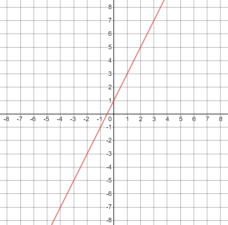
Here are some facts about the equation \(y = 2x+1\):
- When \(x=3\), \(y=7\). You can figure this out in two ways:
- Plug 3 in for x in the equation: \(y = 2(3)+1 = 6+1=7\).
- Find 3 on the x (horizontal) axis in the graph. Draw a vertical line up from \(x=3\) on the x-axis to the line. Then, draw a horizontal line to the y (vertical) axis on the left. This line will hit the y-axis at 7.
- Now let’s increase \(x\) by 1, such that \(x=4\). Then \(y=9\).
- When we increased \(x\) by 1, \(y\) increased by 2.79 So, for this equation, \(m=2\).
- When \(x=0\), \(y=1\). So, for this equation, \(b=1\).
Most importantly, when we describe the relationship between \(y\) and \(x\) above, we phrase it like this: For every one unit increase in x, y increases by 2. During your time in this course, you will be starting many sentences with the words “For every one unit increase…” It is important for you to remember these five words.
Another way to write a linear equation is like this:
\[ y = b_1x + b_0 \]
In the linear equation above:
- \(b_1\) = slope
- \(b_0\) = intercept
- \(y\) is the dependent variable, the outcome we care about
- \(x\) is the independent variable, the input that is associated with the dependent variable
Statistical results and formulas are often written with these \(b_{something}\) coefficients rather than \(m\) and \(b\).
Below, we will make an analogy between the linear equations above and a trend line that can be drawn to fit a set of data.
6.1.2 Linear relationship between variables
Linear equations allow us to figure out the relationship between two variables in a survey data set. That relationship between two variables can be expressed using the same type of linear equation we just reviewed. Before we do that, let’s set up an example. We will look at the mtcars dataset, which is built into R. You can get more information about the mtcars dataset by running the code ?mtcars on your computer. You can also inspect the data by running the code View(mtcars) on your computer.
The mtcars dataset is also displayed below:
mtcars## mpg cyl disp hp drat wt qsec vs am gear carb
## Mazda RX4 21.0 6 160.0 110 3.90 2.620 16.46 0 1 4 4
## Mazda RX4 Wag 21.0 6 160.0 110 3.90 2.875 17.02 0 1 4 4
## Datsun 710 22.8 4 108.0 93 3.85 2.320 18.61 1 1 4 1
## Hornet 4 Drive 21.4 6 258.0 110 3.08 3.215 19.44 1 0 3 1
## Hornet Sportabout 18.7 8 360.0 175 3.15 3.440 17.02 0 0 3 2
## Valiant 18.1 6 225.0 105 2.76 3.460 20.22 1 0 3 1
## Duster 360 14.3 8 360.0 245 3.21 3.570 15.84 0 0 3 4
## Merc 240D 24.4 4 146.7 62 3.69 3.190 20.00 1 0 4 2
## Merc 230 22.8 4 140.8 95 3.92 3.150 22.90 1 0 4 2
## Merc 280 19.2 6 167.6 123 3.92 3.440 18.30 1 0 4 4
## Merc 280C 17.8 6 167.6 123 3.92 3.440 18.90 1 0 4 4
## Merc 450SE 16.4 8 275.8 180 3.07 4.070 17.40 0 0 3 3
## Merc 450SL 17.3 8 275.8 180 3.07 3.730 17.60 0 0 3 3
## Merc 450SLC 15.2 8 275.8 180 3.07 3.780 18.00 0 0 3 3
## Cadillac Fleetwood 10.4 8 472.0 205 2.93 5.250 17.98 0 0 3 4
## Lincoln Continental 10.4 8 460.0 215 3.00 5.424 17.82 0 0 3 4
## Chrysler Imperial 14.7 8 440.0 230 3.23 5.345 17.42 0 0 3 4
## Fiat 128 32.4 4 78.7 66 4.08 2.200 19.47 1 1 4 1
## Honda Civic 30.4 4 75.7 52 4.93 1.615 18.52 1 1 4 2
## Toyota Corolla 33.9 4 71.1 65 4.22 1.835 19.90 1 1 4 1
## Toyota Corona 21.5 4 120.1 97 3.70 2.465 20.01 1 0 3 1
## Dodge Challenger 15.5 8 318.0 150 2.76 3.520 16.87 0 0 3 2
## AMC Javelin 15.2 8 304.0 150 3.15 3.435 17.30 0 0 3 2
## Camaro Z28 13.3 8 350.0 245 3.73 3.840 15.41 0 0 3 4
## Pontiac Firebird 19.2 8 400.0 175 3.08 3.845 17.05 0 0 3 2
## Fiat X1-9 27.3 4 79.0 66 4.08 1.935 18.90 1 1 4 1
## Porsche 914-2 26.0 4 120.3 91 4.43 2.140 16.70 0 1 5 2
## Lotus Europa 30.4 4 95.1 113 3.77 1.513 16.90 1 1 5 2
## Ford Pantera L 15.8 8 351.0 264 4.22 3.170 14.50 0 1 5 4
## Ferrari Dino 19.7 6 145.0 175 3.62 2.770 15.50 0 1 5 6
## Maserati Bora 15.0 8 301.0 335 3.54 3.570 14.60 0 1 5 8
## Volvo 142E 21.4 4 121.0 109 4.11 2.780 18.60 1 1 4 2As you know, survey data are arranged in a spreadsheet, with each row corresponding to an observation and each column corresponding to a characteristic or variable. In this case, the unit of observation is the car, so each row in this data is a car. There are 32 cars in total in the data. A survey-taker surveyed these 32 cars and found out a number of characteristics about them.
Consider this research question: Is a car’s gas efficiency influenced by the number of cylinders it has?
This question is very hard to answer, because we are asking if a car’s cylinders cause its gas efficiency. This question is too hard to answer, so we are going to tackle a slightly easier research question: Is gas efficiency, as measured by miles per gallon (mpg) associated with the number of cylinders (cyl) that a car has?
Now it’s time to see what the statistical relationship is between mpg and cyl, or mpg vs cyl, we could say. We always write [dependent variable] vs [independent variable]. Let’s start with a simple scatterplot:
plot(mtcars$cyl,mtcars$mpg, main = "Scatterplot")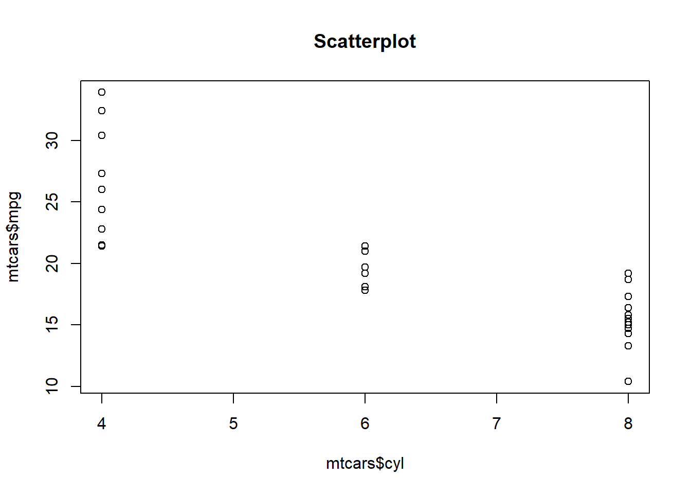
We always put the dependent variable on the y-axis (the vertical axis) and the independent variable on the x-axis (the horizontal axis). Clearly, this plot suggests that there is a noteworthy relationship between mpg and cyl.
Next, we run a linear regression to fit a trend line to this data. At this point in the course, it is not necessary for you to know what exactly a linear regression is. All you need to know for now is that it helped us fit a trend line to the data in our scatterplot above.
Let’s have a look at the scatterplot of our data again, this time including the trendline that we just calculated:
plot(mtcars$cyl,mtcars$mpg, main = "Scatterplot with trendline")
abline(lm(mpg~cyl,data=mtcars))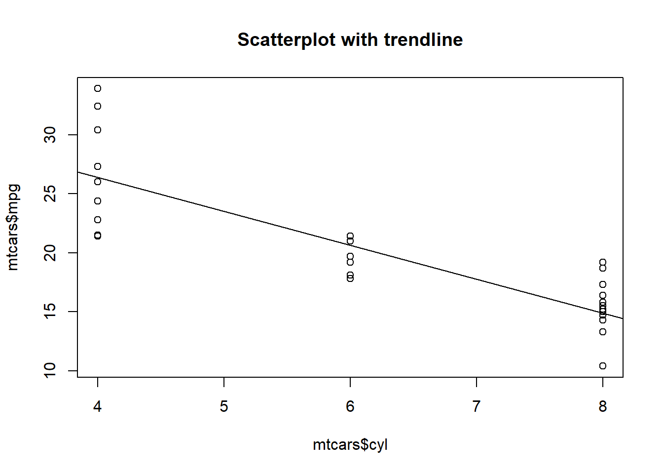
This is where we return to the linear equation. The equation of the trendline is:
\[y = -2.9x+37.9\]
In this example, the variables \(y\) and \(x\) have names other than just \(y\) and \(x\). Let’s rewrite the equation with these new names:
\[mpg = -2.9cyl+37.9\]
In this case, \(y\) is the dependent variable, which is mpg. \(x\) is the independent variable, which is cyl. \(b_1 = -2.9\) and \(b_0 = 37.9\). \(b_1\) is the slope and \(b_0\) is the intercept.
This is how we phrase the results of this regression analysis: For each additional cylinder, a car is predicted to have 2.9 fewer miles per gallon of gas efficiency. It is not a certainty. It is just a prediction. Now, let’s make some more predictions.
We will be interpreting different types of linear equations throughout this course. As we do that, just keep in mind that we are just using slopes to express relationships between dependent and independent variables, the same way we were in the equations and trends that we reviewed above.
6.2 Correlation
Correlation is a basic statistic that we can use to determine the relationship between two variables. A correlation coefficient—commonly written as \(r\)—gives a quantitative measure of how strongly related two variables are or are not. When we discuss correlation in this section, we will imagine that we are interested in the relationship between two variables, X and Y. X and Y can be negatively, zero, or positively correlated.
Here are what these three types of correlations mean:
- Negative Correlation: As variable X increases, variable Y decreases
- Zero Correlation: As variable X increases, we do not know what happens to variable Y.
- Positive Correlation: As variable X increases, variable Y increases
The most common way in which correlation is calculated is called Pearson’s correlation or Pearson’s r. When we use correlation in this book, it will always refer to Pearson’s correlation unless otherwise specified. The terms r, correlation, and correlation coefficient are often used interchangeably; they all mean the same thing.
The correlation coefficient can range from -1 to +1.80
- -1 means that there is a perfect negative relationship between X and Y.
- 0 means that there is no relationship between X and Y.
- +1 means that there is a perfect positive relationship between X and Y.
Here are some examples of correlation:81
| Unit of observation | X variable | Y variable | Correlation | What it means |
|---|---|---|---|---|
| cities | distance from ocean | flood incidents | -0.3 | cities with high distances from the ocean have fewer flood incidents |
| humans | age | distance from Havana | 0 | age is completely unrelated to how far from Havana people live |
| households | annual income | square footage of home | 0.7 | households with high annual incomes have homes with high square footages |
Sometimes, we calculate the square of our correlation coefficient. This is often referred to as \(R^2\), R-squared, R-square, or coefficient of determination. All of these terms mean the same thing. \(R^2\) refers to the proportion (or percentage) of variation in Y that can be accounted for by variation in X. This statistic is commonly used alongside regression analysis.
6.2.1 Calculating and interpreting correlation
Now that you have read a little bit about the concept of correlation, you may find it useful to see a few videos that demonstrate and apply the concept. Note that these videos were created by different instructor(s) for different audiences.
We’ll start with this video that gives an overview of correlation:82
The video above can be viewed externally at https://www.youtube.com/watch?v=qC9_mohleao.
This follow-up video goes into more detail:83
The video above can be viewed externally at https://www.youtube.com/watch?v=ugd4k3dC_8Y.
Finally, the following article provides very clear step-by-step instructions of how to calculate a correlation coefficient by hand:
- wikiHow Staff. How to Find the Correlation Coefficient. wikiHow. March 29, 2019. Click here.
6.2.2 Correlation in R
Let’s turn to calculating correlation in R. To do this, we will just use the built-in dataset mtcars. Let’s create a dataset called d which is a copy of mtcars:
d <- mtcarsWe can inspect our entire dataset d with the following command:
View(d)In this example, we will just focus on the relationship between a car’s weight (wt) and displacement (disp). Keep in mind that each observation in our data set is a separate car (automobile). Note that weight is measured in tons and displacement is measured in cubic inches. Weight is our independent variable of interest and displacement is our dependent variable of interest.
Below, we can inspect our observations (cars) in our data just for these two variables of interest:84
d[c("wt","disp")]## wt disp
## Mazda RX4 2.620 160.0
## Mazda RX4 Wag 2.875 160.0
## Datsun 710 2.320 108.0
## Hornet 4 Drive 3.215 258.0
## Hornet Sportabout 3.440 360.0
## Valiant 3.460 225.0
## Duster 360 3.570 360.0
## Merc 240D 3.190 146.7
## Merc 230 3.150 140.8
## Merc 280 3.440 167.6
## Merc 280C 3.440 167.6
## Merc 450SE 4.070 275.8
## Merc 450SL 3.730 275.8
## Merc 450SLC 3.780 275.8
## Cadillac Fleetwood 5.250 472.0
## Lincoln Continental 5.424 460.0
## Chrysler Imperial 5.345 440.0
## Fiat 128 2.200 78.7
## Honda Civic 1.615 75.7
## Toyota Corolla 1.835 71.1
## Toyota Corona 2.465 120.1
## Dodge Challenger 3.520 318.0
## AMC Javelin 3.435 304.0
## Camaro Z28 3.840 350.0
## Pontiac Firebird 3.845 400.0
## Fiat X1-9 1.935 79.0
## Porsche 914-2 2.140 120.3
## Lotus Europa 1.513 95.1
## Ford Pantera L 3.170 351.0
## Ferrari Dino 2.770 145.0
## Maserati Bora 3.570 301.0
## Volvo 142E 2.780 121.0Next, let’s create a scatterplot of these two variables. We’ll put our outcome of interest on the vertical axis and our input of interest on the horizontal axis.
plot(d$wt, d$disp)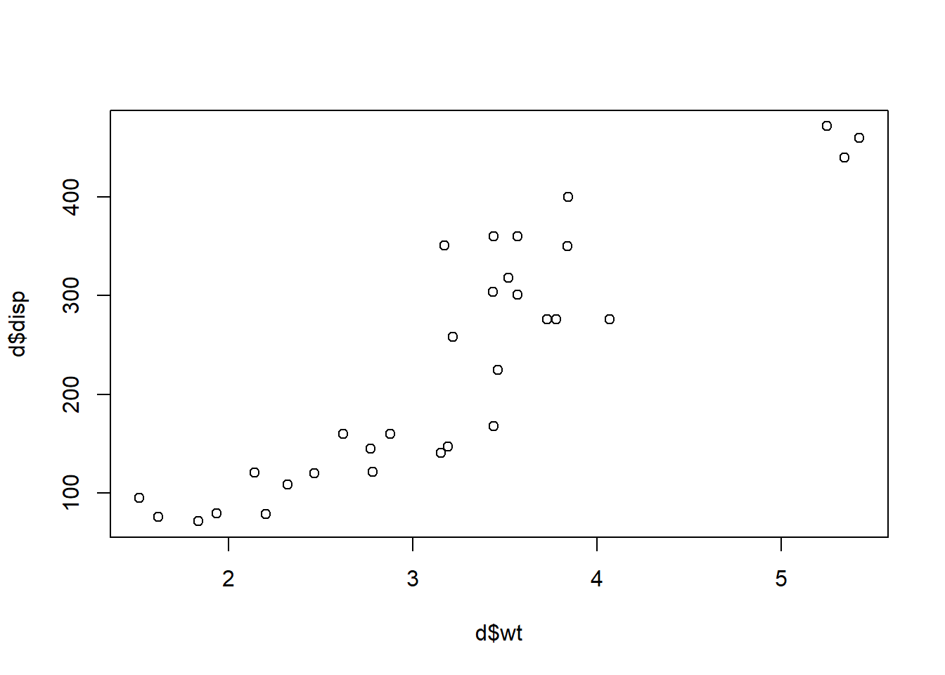
Just by visually inspecting the scatterplot above, you can see that there appears to be a close association between weight and displacement of a car in our sample. We are now ready to calculate the correlation of weight and displacement.
The code below calculates correlation in R:
cor(d$wt,d$disp)## [1] 0.8879799Here is what we asked the computer to do for us above:
cor(...)– Calculate the correlation between two variables, X and Y.d$wt– X variable.d$disp– Y variable.
As you can see, the correlation between weight and displacement is 0.89. This is a very high correlation. This means that cars with heavy weight are likely to also have high displacement.
We can save this calculated correlation in R’s memory in case we want to use it later:
r <- cor(d$wt,d$disp)Above, we created the object r which saves the result of the code cor(d$wt,d$disp). You will notice that r now appears as a stored object within your environment in RStudio.
We can run the code r and the computer will show us that it did indeed store this for us:
r## [1] 0.8879799Above, we ran the command r and the computer responded to us by showing us that it stored 0.89 as r.
We can also calculate \(R^2\) with the code below:
r^2## [1] 0.7885083Above, the computer is telling us that \(R^2 = 0.79\), which is the square of 0.89.
You are now equipped to calculate and interpret correlations in R.
6.2.3 Correlation matrix in R
If we want to see correlations for multiple variables within a dataset all at once, we can create a correlation matrix.85 A correlation matrix can sometimes be large and difficult to read if we include all of the variables in a particular dataset in our matrix. A more straightforward approach is to create a separate dataset which includes only the variables for which you want to see correlations.
Here we make a partial dataset of mtcars called mtcars.partial:86
mtcars.partial <- mtcars[c("disp","wt","drat", "am")]Our new dataset called mtcars.partial contains the variables disp, wt, drat, and am from our original mtcars dataset.
Now we can make a correlation matrix on the dataset mtcars.partial:
cor(mtcars.partial)## disp wt drat am
## disp 1.0000000 0.8879799 -0.7102139 -0.5912270
## wt 0.8879799 1.0000000 -0.7124406 -0.6924953
## drat -0.7102139 -0.7124406 1.0000000 0.7127111
## am -0.5912270 -0.6924953 0.7127111 1.0000000In the output above, we see pairwise correlations for each combination of variables in our dataset. For example, disp and drat are correlated at -0.71.
A correlation matrix can help us quickly look for associations between variables in our data.
6.3 Assignment
In this assignment, you will practice using linear equations, calculate a correlation coefficient by hand, and use R to do a short correlation-based study.
6.3.1 Linear relationships
Now we will turn to a review of linear relationships. Some of the tasks below relate to datasets that you have encountered earlier in this chapter and others relate more conceptually to linear relationships.
You can write down your answers anywhere you would like and then submit them as a separate file in D2L. For example, you can write your answers to this part of the assignment in a Microsoft Word document. Then, you would submit both the Word document and your R script file from above (two files total) in D2L.
Task 1: Draw a small coordinate plane (graph) on a paper. Graph the line represented by the equation \(y = -1.5x+5\). When \(x = 2\), what is \(y\)? Plug 2 into the equation in place of x to figure it out! Show all of your work.
Task 2: In the same equation, \(y = -1.5x+5\), what is \(y\) when \(x=3\)?
Task 3: For the equation \(y = -1.5x+5\), how do you express the relationship between \(y\) and \(x\)? Make sure your answer begins with the five important words “For every one unit increase…”87
Task 4: In the equation \(y = -1.5x+5\), what is the dependent variable and what is the independent variable?
Task 5: Earlier in the chapter, we found that the predicted relationship between mpg and cyl in the mtcars data is described by the equation \(mpg = -2.9cyl+37.9\). In this equation, what is the dependent variable and what is the independent variable?
Task 6: Based on the equation \(mpg = -2.9cyl+37.9\), if a car has 4 cylinders, what is its predicted fuel efficiency? Show each step of your work.
Task 7: Based on the equation \(mpg = -2.9cyl+37.9\), if a car has 3 cylinders, what is its predicted fuel efficiency? Show your work.
Task 8: What is the difference in predicted mpg for a car with 4 cylinders compared to a car with 3 cylinders? What is another name for this difference, in the terminology of linear equations?
Task 9: Interpret the number -2.9 from the equation \(mpg = -2.9cyl+37.9\). Be sure to use the five important words as part of your answer!
6.3.2 Correlation Calculation Practice
Look at the following fitness dataset containing five people:
WeeklyWeightliftHoursis the number of hours per week the person spends weightlifting.WeightLiftedKGis how much weight the person could lift on the day of the survey.
Name <- c("Person A","Person B","Person C","Person D","Person E")
WeeklyWeightliftHours <- c(3,4,4,2,6)
WeightLiftedKG <- c(20,30,21,25,40)

fitness <- data.frame(Name, WeeklyWeightliftHours, WeightLiftedKG)
fitness
## Name WeeklyWeightliftHours WeightLiftedKG
## 1 Person A 3 20
## 2 Person B 4 30
## 3 Person C 4 21
## 4 Person D 2 25
## 5 Person E 6 40Task 10: What is a reasonable research question that we could ask with this data?
Task 11: What is the dependent variable and independent variable for a quantitative analysis that we could do to answer this research question?
Task 12: What is the correlation coefficient for WeightLiftedKG and WeeklyWeightliftHours? Show all of your work/calculations. Please calculate this manually, not using R.
Here’s the answer, but you still need to make sure you do and show the work correctly:
# Calculate correlation between two vectors/variables
CorrelationWeightHours <- cor(fitness$WeeklyWeightliftHours,fitness$WeightLiftedKG)
CorrelationWeightHours
## [1] 0.7677303And here’s what it looks like visually:
plot(fitness$WeeklyWeightliftHours,fitness$WeightLiftedKG)
reg1 <-  lm(fitness$WeightLiftedKG~fitness$WeeklyWeightliftHours)
abline(reg1)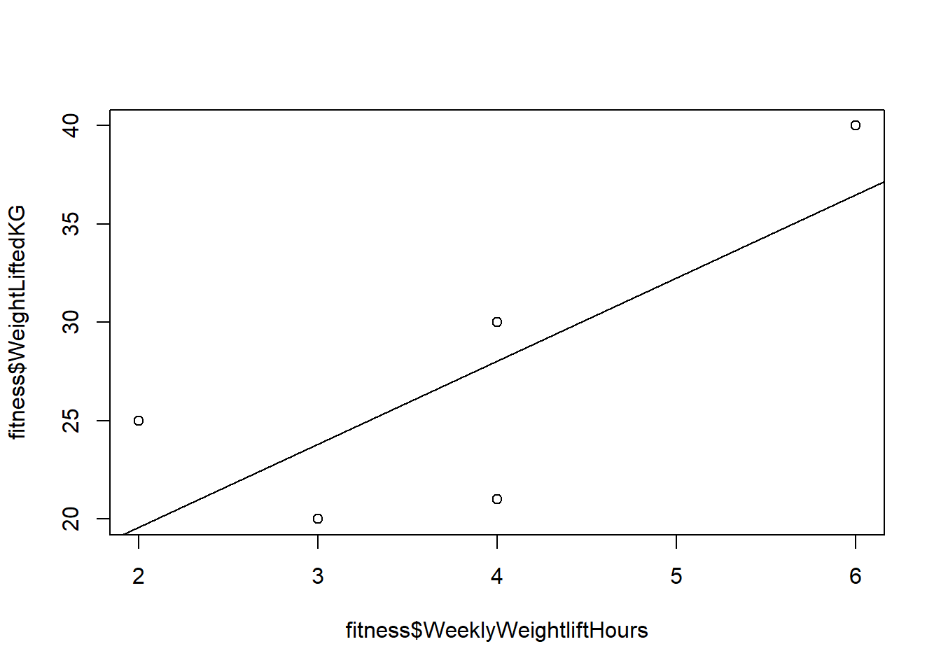
6.3.3 Correlation Study
For this part of the assignment, you’ll need to use the bodyfat.sav dataset available here. This is an SPSS format dataset, so you’ll have to load it using the following code:
if (!require(foreign)) install.packages('foreign')
library(foreign)
bf <- read.spss("bodyfat.sav", to.data.frame = TRUE)
Information about the data: Data are taken from a study examining the relationships between body measurements and weight among physically active adults. You will be working with a subset of the data containing 252 men. Skeletal measurements were taken for 9 different areas of the body (chest-wrist in dataset). The dataset also contains age, height, and weight.
Note that bf is the name of the dataset you imported with the code above. You should refer to it as bf in your R code.
If you prefer, or if it would be more productive for your work, you are welcome to use data of your own (instead of the bodyfat.sav dataset) to do this portion of the assignment, as long as it contains enough continuous numeric variables for you to do the tasks below.
Task 13: Familiarize yourself with the dataset. Calculate descriptive statistics, grouped descriptive statistics, and/or one-way or two-way tables, where appropriate. You can also create visualizations that may help you explore the data.
Task 14: In looking at the variables in the dataset, make some hypotheses about which variables might be related (or more related, compared to others) to weight. Write out your hypotheses.
Task 15: Test your hypotheses with correlations. Calculate correlations between height, weight, and the nine body measurements. Create a correlation matrix88 to do this. Which hypotheses seem to be supported by the correlations?
Task 16: Create a scatterplot for one of the relationships that you hypothesized about above.
Task 17: Write a short paragraph with any conclusions and limitations of what you found. Approximately five sentences will be sufficient.
6.3.4 Follow up and submission
You have now reached the end of this week’s assignment. The tasks below will guide you through submission of the assignment and allow us to gather questions and/or feedback from you.
Task 18: Please write any questions you have for the course instructors (optional).
Task 19: Please write any feedback you have about the instructional materials (optional).
Task 20: If you have not done so already, please e-mail Nicole and Anshul to schedule your Oral Exam #1.
Task 21: Please submit your assignment (multiple files are fine) to the D2L assignment drop-box corresponding to this chapter and week of the course. Please e-mail all instructors if you experience any difficulty with this process.
Produced using the graphing calculator at https://www.desmos.com/calculator.↩︎
Remember: when x was 3, y was 7. When we increased x to 4, y became 9. y changed from 7 to 9, which means that it increased by 2 when we increased x by 1.↩︎
It is never lower than -1 and never higher than +1.↩︎
All of these examples and numbers are hypothetical and not based on empirical data of any kind. They are for illustrative purposes only.↩︎
Correlation - The Basic Idea Explained. Benedict K. Apr 11, 2014. YouTube. https://www.youtube.com/watch?v=qC9_mohleao.↩︎
The Correlation Coefficient - Explained in Three Steps. Benedict K. May 1, 2014. YouTube. https://www.youtube.com/watch?v=ugd4k3dC_8Y.↩︎
An explanation of this code can be found in the section on subsetting datasets by variable names.↩︎
This section was added on February 25 2021. It was accidentally omitted prior to this date.↩︎
We could have called it anything else that we wanted. It does not have to necessarily have
partialin its name.↩︎Hint: Look at your answers to the previous two questions. What was the value of y when x was 2? What was the new value of y when you changed x to 3? What is the difference between these two values of y? That difference is the change in y for every one-unit change in x.↩︎
When this chapter was initially published, the section on how to make a correlation matrix in R was accidentally omitted. It has been added to this chapter on February 25 2021.↩︎