Chapter 15 Linear Relationships
This chapter is not part of the course HE802 in spring 2021.
15.1 Answers To Your Questions, Tips, and Tricks
Here are answers to some of your questions that might be helpful for everyone to see. A lot of these answers contain tips and tricks that might help you explore or analyze your data. You are not required to read these.
15.1.1 Oral Exams
How should I prepare for the oral exam? What exactly will it test?
- The exam will mostly test you knowledge of the statistical methods we have learned so far (before February 10, 2020).
- The exam will test you ability to conduct some but not all of these methods in R.
- You can refer to any materials you would like (course book, your notes and assignments, online sources, etc) during the test. Therefore, I suggest that you refresh your memory about where you can find R code that you need, so that you can copy and paste it easily. Beyond that I recommend reviewing the statistical concepts more than R code.
- More weight will be given to your knowledge of statistical concepts than R code.
What will happen during the exam?
- I will ask you a few theoretical questions.
- I will ask you to open a dataset in R and run a few commands in it.
- I will tell you after each question if you were correct or not. You can re-try some tasks on the spot if you wish. Other items can be flagged for re-testing later.
- If you need to have anything re-tested, we can schedule a separate time for that or I can try to include it in Oral Exam #2 in a few weeks, to streamline the process for you.
- We will try to be efficient during the oral exam so that we don’t run out of time.
15.1.2 Converting Categorical and Numeric Data
The following code converts a numeric variable to a categorical one:
DataSet$NewVariable <- as.factor(DataSet$OldVariable)The following code converts a categorical variable to a numeric one:
DataSet$NewVariable <- as.numeric(as.character(DataSet$OldVariable))15.1.3 Converting Time Variables in R
At least one of you has data in which there are time stamps which you need to convert into a continuous variable that you can put into a regression. For example, maybe you have data in which each row (observation) is a patient and then you have a variable (column) for the date and time on which the patient came into the hospital. To analyze this data as a continuous variable, maybe you want to calculate how many seconds after midnight in each day a patient came in.
How can we convert a time to a number of seconds? There are helper functions in R that help us do this. Let’s start with an example:
if (!require(lubridate)) install.packages('lubridate') ## Loading required package: lubridate##
## Attaching package: 'lubridate'## The following objects are masked from 'package:base':
##
## date, intersect, setdiff, unionlibrary(lubridate) # this package has the period_to_seconds function
# example of what the data looks like
ExampleTimestamp <- "01-01-2019 09:04:58"
# extract just the time (remove the date)
(ExampleTimeOnly <- substr(ExampleTimestamp,12,19))## [1] "09:04:58"# convert from time to number of seconds
(TotalSeconds <- period_to_seconds(hms(ExampleTimeOnly)))## [1] 32698As you can see above, the time “09:04:59” was converted into 32698 seconds. But we only did it for a single stored value, ExampleTimestamp. How do we do it for the entire variable in a dataset? Let’s say you have a datset called d with a variable with a time stamp called timestamp and you want to make a new variable (column) in the dataset called seconds. Here’s how you can do it:
if (!require(lubridate)) install.packages('lubridate')
library(lubridate)

d$seconds <- period_to_seconds(hms(substr(d$timestamp,12,19)))
15.1.4 Load Packages Easily
The code below will load a package if it is already installed and install it if it is not already installed. The example below is for the car package. You will have to replace the word “car” in the code below with the name of the package you want to use.
if (!require(car)) install.packages('car')## Loading required package: car## Loading required package: carDatalibrary(car)The second line isn’t always needed but it doesn’t hurt to just put it in there.
15.1.5 Assigning New Values in R
Here’s how you make a copy of anything in R:
thing1 <- thing2The code above is doing the following:
- Create a new object called
thing1 - The
<-operator assigns whatever is on the right to whatever is on the left. - Assign
thing1to be the value ofthing2.thing2still exists too, note.
Some of you have done this for your assignments with the data we have been using:
d <- GSSvocab
This makes a copy of GSSvocab called d. Then you can just use this dataset without having to type GSSvocab each time.
15.1.6 Console Versus RMarkdown File
In general, all commands should go into your RMarkdown file which is likely in the top-left of your RStudio screen. This way, you have them saved for later when you want to replicate your work or copy the code you used to use again with different data.
However, there are at least two exceptions. The following two commands should never be put in the RMarkdown file and only be run directly in the console:
View(YourDataName)– This is the command you use to view your data in spreadsheet form, within R.file.choose()– This is the command you can use to get the exact file path of a file or folder.
These commands cannot go into your RMarkdown file. Most of you will “Knit” your RMarkdown file into a PDF file to submit/publish your work. But the View command requires a separate window to open in RStudio to show you a spreadsheet. This separate spreadsheet window can’t open in a PDF! You wouldn’t want your entire dataset to show up in the PDF in spreadsheet form, would you? No. You just want the results of the other commands you run to show up. That’s why you get an error if you include the View command in your RMarkdown file and you try to Knit it.
15.2 Correlation
Have a look at these resources:
A correlational analysis is an analytic method for assessing the relationship between two variables. A correlation coefficient (r) provides a description of the relationship between the two variables, and suggests an inference. For example, the correlation between footprint size and height is .8. The inference from this correlation is that “If someone has big footprints, he is probably tall.”
Positive Correlation: As variable X increases, variable Y increases
Negative Correlation: As variable X increases, variable Y decreases
The most common index of the relationship between two continuous variables is Pearson’s r. Pearson’s r represents the strengths of the correlation.
r can range from -1 to 1:
- -1 and +1 reflects a perfect relationship between two variables
- 0 reflects no relationship between two variables
r indicates the direction of relationship:
- r can be positive (+) or negative (-)
- A positive correlation means that as one variable increases, the other also increases
- A negative correlation means that as one variable increases, the other decreases
There are a few other types of correlation coefficients you should be aware of:
- Spearman’s rho: when you have two ordinal variables
- Kendall’s tau: when you have two ordinal variables
- Point-biserial correlation: When one variable is continuous and the other is dichotomous
Coefficient of Determination, \(R^2\): Percentage of variability of Y accounted for by X; usually used in the context of regression, but can be used for simple correlation as well. Simply square Pearson’s r to get the percentage of variability X accounts for in variable Y.
Partial Correlation: If three variables are all correlated with one another, but you are interested in understanding the unique relationship between two of those variables, you need to control for the effects of the third variable. A partial correlation allows you to look at the relationship between two variables, controlling for the effects of a third variable.
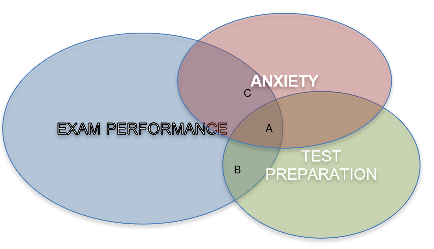
A = variance in exam performance accounted for by BOTH anxiety and test preparation
B = variance in exam performance accounted for by test preparation
C = variance in exam performance accounted for by anxiety
If you were to ignore the effect of test preparation, you would overestimate the relationship between exam performance and anxiety (it would equal A + C). By controlling for A, you can estimate the unique relationship between exam performance and anxiety (C).
15.2.1 Calculating Correlation
The following resources can help you calculate correlation:
- wikiHow Staff. How to Find the Correlation Coefficient. wikiHow. March 29, 2019. https://www.wikihow.com/Find-the-Correlation-Coefficient#targetText=To%20find%20the%20correlation%20coefficient%20by%20hand%2C%20first%20put%20your,Y%20in%20the%20same%20way.
- Calculating correlation coefficient r. July 11 2017. Khan Academy. https://www.youtube.com/watch?v=u4ugaNo6v1Q.
- Benedict K. The Correlation Coefficient - Explained in Three Steps. May 1 2014. https://www.youtube.com/watch?v=ugd4k3dC_8Y.
15.2.2 Correlation in R
This is how you can calculate correlations in R:
And this is how you can make a correlation matrix:
cor(mtcars[c("mpg","cyl","hp","gear")])## mpg cyl hp gear
## mpg 1.0000000 -0.8521620 -0.7761684 0.4802848
## cyl -0.8521620 1.0000000 0.8324475 -0.4926866
## hp -0.7761684 0.8324475 1.0000000 -0.1257043
## gear 0.4802848 -0.4926866 -0.1257043 1.0000000Above, we are selecting four variables from the dataset mtcars and we are looking at their correlations.
If we also want p-values, we can do the following:
if (!require(Hmisc)) install.packages('Hmisc') ## Loading required package: Hmisc## Loading required package: lattice## Loading required package: survival## Loading required package: Formula## Loading required package: ggplot2##
## Attaching package: 'Hmisc'## The following objects are masked from 'package:base':
##
## format.pval, unitslibrary(Hmisc)
cor1 <- rcorr(as.matrix(mtcars[c("mpg","cyl","hp","gear")]))
cor1## mpg cyl hp gear
## mpg 1.00 -0.85 -0.78 0.48
## cyl -0.85 1.00 0.83 -0.49
## hp -0.78 0.83 1.00 -0.13
## gear 0.48 -0.49 -0.13 1.00
##
## n= 32
##
##
## P
## mpg cyl hp gear
## mpg 0.0000 0.0000 0.0054
## cyl 0.0000 0.0000 0.0042
## hp 0.0000 0.0000 0.4930
## gear 0.0054 0.0042 0.493015.3 Scatterplots
See these examples:
Scatterplots are a tool you can use to visualize and identify the nature of the relationship between two variables. A scatterplot plots values of one variable against those of the other. You should be able to look at a scatterplot and estimate the size and direction of the relationship between two variables. Scatterplots can be created in any statistical software package.
If you want, try making up your own data for two variables. Plot the data using a scatterplot. After examining your plot, estimate what you think the correlation is between the two variables. Then, calculate r. How close was your guess? Try changing a few values in your dataset and see what happens to your plot/correlation.
Here’s how you make a scatterplot in R:
I usually just use the plot command:
plot(DatasetName$X_Variable, DatasetName$Y_Variable)15.4 Assignment
15.4.1 Linear Relationships Review
\[ y = mx + b \]
Remember this? This is a linear equation in which
\[m = slope\] \[b = intercept\]
Task 1: Draw a small coordinate plane (graph) on your paper. Graph the equation \(y = 2x + 1\). When x = 7, what is y? Plug 7 into the equation in place of x to figure it out! Show all of your work.
Task 2: On the same coordinate plane, graph the equation \(y = 0.5x + 3\). As x increases by one unit, what happens to y? When x = 7, what is y?
Now I’m going to rewrite the formula for a linear equation:
\[ y = b_1 x+b_0\]
In this new version, \(b_1\) is the slope and \(b_0\) is the intercept. Statistical results and formulas are often written with these \(b_{whatever}\) coefficients rather than \(m\).
Linear equations allow us to figure out the relationship between two variables in a survey data set. Let’s look at this data on cars:
mtcars## mpg cyl disp hp drat wt qsec vs am gear carb
## Mazda RX4 21.0 6 160.0 110 3.90 2.620 16.46 0 1 4 4
## Mazda RX4 Wag 21.0 6 160.0 110 3.90 2.875 17.02 0 1 4 4
## Datsun 710 22.8 4 108.0 93 3.85 2.320 18.61 1 1 4 1
## Hornet 4 Drive 21.4 6 258.0 110 3.08 3.215 19.44 1 0 3 1
## Hornet Sportabout 18.7 8 360.0 175 3.15 3.440 17.02 0 0 3 2
## Valiant 18.1 6 225.0 105 2.76 3.460 20.22 1 0 3 1
## Duster 360 14.3 8 360.0 245 3.21 3.570 15.84 0 0 3 4
## Merc 240D 24.4 4 146.7 62 3.69 3.190 20.00 1 0 4 2
## Merc 230 22.8 4 140.8 95 3.92 3.150 22.90 1 0 4 2
## Merc 280 19.2 6 167.6 123 3.92 3.440 18.30 1 0 4 4
## Merc 280C 17.8 6 167.6 123 3.92 3.440 18.90 1 0 4 4
## Merc 450SE 16.4 8 275.8 180 3.07 4.070 17.40 0 0 3 3
## Merc 450SL 17.3 8 275.8 180 3.07 3.730 17.60 0 0 3 3
## Merc 450SLC 15.2 8 275.8 180 3.07 3.780 18.00 0 0 3 3
## Cadillac Fleetwood 10.4 8 472.0 205 2.93 5.250 17.98 0 0 3 4
## Lincoln Continental 10.4 8 460.0 215 3.00 5.424 17.82 0 0 3 4
## Chrysler Imperial 14.7 8 440.0 230 3.23 5.345 17.42 0 0 3 4
## Fiat 128 32.4 4 78.7 66 4.08 2.200 19.47 1 1 4 1
## Honda Civic 30.4 4 75.7 52 4.93 1.615 18.52 1 1 4 2
## Toyota Corolla 33.9 4 71.1 65 4.22 1.835 19.90 1 1 4 1
## Toyota Corona 21.5 4 120.1 97 3.70 2.465 20.01 1 0 3 1
## Dodge Challenger 15.5 8 318.0 150 2.76 3.520 16.87 0 0 3 2
## AMC Javelin 15.2 8 304.0 150 3.15 3.435 17.30 0 0 3 2
## Camaro Z28 13.3 8 350.0 245 3.73 3.840 15.41 0 0 3 4
## Pontiac Firebird 19.2 8 400.0 175 3.08 3.845 17.05 0 0 3 2
## Fiat X1-9 27.3 4 79.0 66 4.08 1.935 18.90 1 1 4 1
## Porsche 914-2 26.0 4 120.3 91 4.43 2.140 16.70 0 1 5 2
## Lotus Europa 30.4 4 95.1 113 3.77 1.513 16.90 1 1 5 2
## Ford Pantera L 15.8 8 351.0 264 4.22 3.170 14.50 0 1 5 4
## Ferrari Dino 19.7 6 145.0 175 3.62 2.770 15.50 0 1 5 6
## Maserati Bora 15.0 8 301.0 335 3.54 3.570 14.60 0 1 5 8
## Volvo 142E 21.4 4 121.0 109 4.11 2.780 18.60 1 1 4 2Survey data are arranged in a spreadsheet, with each row corresponding to an observation and each column corresponding to a characteristic or variable. In this case, the unit of observation is the car, so each row in this data is a car. There are 32 cars in total in the data. A survey-taker surveyed these 32 cars and found out a number of characteristics about them.
Task 3: What was the unit of observation in the data on height that you saw earlier in this assignment?
Consider this research question: Is a car’s gas efficiency influenced by the number of cylinders it has?
This question is very hard to answer, because we are asking if a car’s cylinders cause its gas efficiency. This question is too hard to answer, so we are going to tackle a slightly easier research question: Is gas efficiency, as measured by miles per gallon (mpg) associated with the number of cylinders (cyl) that a car has?
Task 4: What is the dependent variable in this research question?
Task 5: What is the independent variable in this research question?
Remember: the dependent variable depends upon the independent variable. The independent variable doesn’t depend on anything; it’s independent and can do whatever it “wants.”
Now it’s time to see what the statistical relationship is between mpg and cyl, or mpg vs cyl, we could say. We always write [dependent variable] vs [independent variable]. Let’s start with a simple scatterplot:
plot(mtcars$cyl,mtcars$mpg)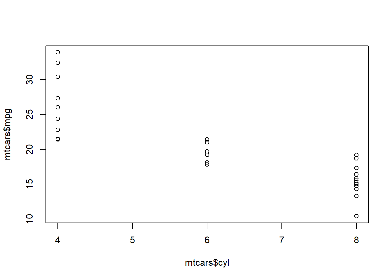
We always put the dependent variable on the y-axis (the vertical axis) and the independent variable on the x-axis (the horizontal axis). Clearly, this plot suggests that there is a noteworthy relationship between mpg and cyl.
Next, we run a linear regression on these two variables in this data:
summary(lm(mpg~cyl,data=mtcars))##
## Call:
## lm(formula = mpg ~ cyl, data = mtcars)
##
## Residuals:
## Min 1Q Median 3Q Max
## -4.9814 -2.1185 0.2217 1.0717 7.5186
##
## Coefficients:
## Estimate Std. Error t value Pr(>|t|)
## (Intercept) 37.8846 2.0738 18.27 < 2e-16 ***
## cyl -2.8758 0.3224 -8.92 6.11e-10 ***
## ---
## Signif. codes: 0 '***' 0.001 '**' 0.01 '*' 0.05 '.' 0.1 ' ' 1
##
## Residual standard error: 3.206 on 30 degrees of freedom
## Multiple R-squared: 0.7262, Adjusted R-squared: 0.7171
## F-statistic: 79.56 on 1 and 30 DF, p-value: 6.113e-10This is where we get back to the linear equation. This regression analysis output is just a linear equation:
\[mpg = -2.9cyl+37.9\]
Remember:
\[ y = b_1 x+b_0 \]
In this case, \(y\) is the dependent variable, which is mpg. \(x\) is the independent variable, which is cyl. \(b_1 = -2.9\) and \(b_0 = 37.9\). \(b_1\) is the slope and \(b_0\) is the intercept.
This is how we phrase the results of this regression analysis: For each additional cylinder, a car is predicted to have 2.9 fewer miles per gallon of gas efficiency. It is not a certainty. It is just a prediction. Now, let’s make some more predictions.
Task 6: If a car has 8 cylinders, what is its predicted gas efficiency? Show each step of your work.186
Task 7: If a car has 4 cylinders, what is its predicted gas efficiency? Show your work.
15.4.2 Correlation Calculation Practice
Look at the following fitness dataset containing five people:
WeeklyWeightliftHoursis the number of hours per week the person spends weightlifting.WeightLiftedKGis how much weight the person could lift on the day of the survey.
Name <- c("Person A","Person B","Person C","Person D","Person E")
WeeklyWeightliftHours <- c(3,4,4,2,6)
WeightLiftedKG <- c(20,30,21,25,40)

fitness <- data.frame(Name, WeeklyWeightliftHours, WeightLiftedKG)
fitness
## Name WeeklyWeightliftHours WeightLiftedKG
## 1 Person A 3 20
## 2 Person B 4 30
## 3 Person C 4 21
## 4 Person D 2 25
## 5 Person E 6 40Task 8: What is a reasonable research question that we could ask with this data?
Task 9: What is the dependent variable and independent variable for a quantitative analysis that we could do to answer this research question?
Task 10: What is the correlation coefficient for WeightLiftedKG and WeeklyWeightliftHours? Show all of your work/calculations.
Here’s the answer, but you still need to make sure you do and show the work correctly:
# Calculate correlation between two vectors/variables
CorrelationWeightHours <- cor(fitness$WeeklyWeightliftHours,fitness$WeightLiftedKG)
CorrelationWeightHours
## [1] 0.7677303And here’s what it looks like visually:
plot(fitness$WeeklyWeightliftHours,fitness$WeightLiftedKG)
reg1 <-  lm(fitness$WeightLiftedKG~fitness$WeeklyWeightliftHours)
abline(reg1)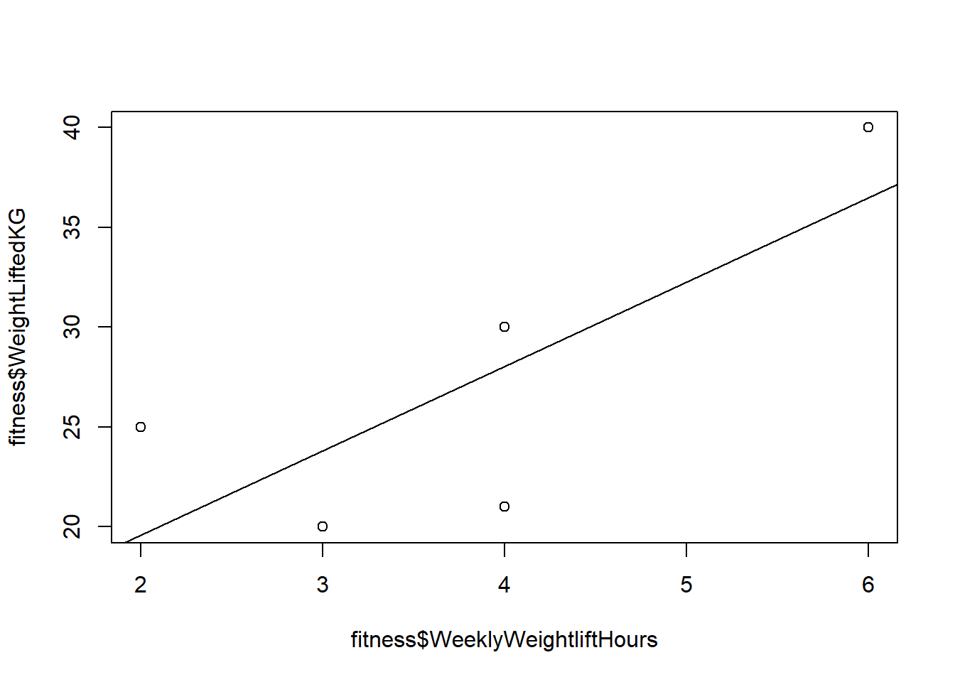
15.4.3 Correlation Study
For this part of the assignment, you’ll need to use the bodyfat.sav dataset available here. This is an SPSS format dataset, so you’ll have to load this using the following code:
if (!require(foreign)) install.packages('foreign')
library(foreign)
bf <- read.spss("bodyfat.sav", to.data.frame = TRUE)
Information about the data: Data are taken from a study examining the relationships between body measurements and weight among physically active adults. You will be working with a subset of the data containing 252 men. Skeletal measurements were taken for 9 different areas of the body (chest-wrist in dataset). The dataset also contains age, height, and weight.
Task 11: Familiarize yourself with the dataset. Calculate descriptive statistics and frequencies, where appropriate. Create a table to summarize the descriptive statistics for the sample and the variables in the dataset.
Task 12: In looking at the variables in the dataset, make some hypotheses about which variables might be related (or more related, compared to others) to weight. Write out your hypotheses.
Task 13: Test your hypotheses with correlations. Calculate correlations between height, weight, and the 9 body measurements. Create a correlation matrix to do this. Make sure that your correlation matrix includes p-values. Which hypotheses seem to be supported by the correlations?
Task 15: Create a scatterplot for one of the relationships that you hypothesized about above.
15.4.4 Final Project Brainstorming
As part of this course, you will have to complete a final project. This project will require you to pick a dataset that already exists (which can be one that you already have and plan to do research upon), identify a research question that you can investigate using that data, and conduct a statistical analysis to answer the question. You will need to provide a brief write-up of your work, as if you are writing only the methods section and results section of a short academic research paper.
This portion of this assignment is meant to help you prepare for this project.
Task 16: What data do you want to use for your project? If you have data of your own, explain the data that you have in 3–6 sentences. Make sure you describe the key variables in the data and mention how many observations are in the data. If you do not have data of your own, brainstorm about what data you could use or let me know that you would like me to provide some for you.
Task 17: What research question would you investigate using the data you specified above? If you do not yet have a datset selected, you do not need to answer this question (and we should meet to discuss which data you could use).
Task 18: What is your hypothesis about the answer to the research question above? If you do not have a research question yet, brainstorm about the types of questions you might be interested in asking, so that I can then think about which already-existing data would be appropriate for your project.
15.4.5 Logistical Tasks
Task 19: Include any questions you have that you wrote down as you read the chapter and did the assignment this week.
Task 20: Please submit your assignment to the online dropbox in D2L as a PDF or HTML file (which you created using RMarkdown187). Please use the same file naming procedure that we used for the previous assignments.
Task 21: Please submit your assignment to me by email.