Chapter 16 OLS Linear Regression
This chapter is not part of the course HE802 in spring 2021.
Last week, we began to use regression analysis to find trends between a dependent variable, an outcome of interest, and an independent variable. This week, we will add multiple independent variables to a linear regression model, so that we can simultaneously see how each one is associated with the dependent variable (while controlling for the other independent variables).
Then, we will examine the assumptions of the ordinary least squares linear regression model. Every time you run a regression analysis (or any statistical test), you need to make sure that your data and your fitted model meet all of the required assumptions of that model/test. Therefore, being able to test those assumptions easily is a critical skill to develop. So, we will practice that skill this week.
This week, our goals are to…
- Run and interpret the result of an OLS (ordinary least squares) linear regression with multiple independent variables.
- Run and interpret the results of diagnostic tests to test the assumptions of OLS linear regression.
16.1 Tips, Tricks, and Answers From Last Week
As always, reading this section is optional, but it is based on questions I received from members of the class over the last week and it may contain some useful information.
16.1.1 All Possible Packages
One of you asked a very good question about packages: Is it possible to see a list of all packages available in R?
Technically, a list is available. This is probably most but not all available packages:
However, there are too many packages listed for the list above to be meaningful to you and me as HPEd researchers who are using R for a vary narrow subset of its full capability. My recommendation is that you identify which task you need to execute and then work backwards from there. If you need to recode data or select variables from a dataset, maybe you use the dplyr package to accomplish this task. If you need to look at residual plots, maybe you use the car package to accomplish this. Hopefully, you can keep this course book as a reference, even after the course is over. Any time you need to do a task that we learned in our course, you can look it up in the book, and the packages that you need to install to perform that task should also be included in the code you see. You will also notice that most of the external resources that we use in this course also tell you which packages you need at the start of the tutorial/explanation.
Additionally, there are web pages that list the packages that the author thinks are most useful. But you will see that this is highly subjective and variable:
- List of R Packages – Master all the Core Packages of R Programming!
- Quick list of useful R packages – This one is from RStudio
- Top 100 R packages for 2013 (Jan-May)! – This appears to be based on empirical data on the most frequently used R packages, rather than being a subjective list.
And finally, here is a list of some of the most important packages we have used so far in our class (or will use soon):
ggpubr
dplyr
expss
plyr
xlsx
car
interactions
foreign
Those are most but not all of the packages we have used so far. I left out the ones that we don’t use as much or that were used in response to a very narrow, specific question (such as the fastDummies package).
16.2 Multiple Linear Regression
16.2.1 Basic Code
Last week, we looked as simple linear regression, with one dependent variable an one independent variable. This week, we will add independent variables to a regression model, such that there is still one dependent variable but multiple independent variables.
Here is the code we introduced and used last week:
reg1 <- lm(DepVar ~ IndVar, data = mydata)
And this week, to add more independent variables, we’ll do it like this:
reg2 <- lm(DepVar ~ IndVar1 + IndVar2 + IndVar3, data = mydata)
Here is what the code above means, which is very similar to last week:
reg2– Create a new regression object calledreg2. You can call this whatever you want. It doesn’t need to be calledreg2.<-– Assignreg2to be the result of the output of the functionlm()lm()– Run a linear model using OLS linear regression.DepVar– This is the dependent variable in the regression model. You will write the name of your own dependent variable instead ofDepVar.~– This is part of a formula. This is like the equals sign within an equation.IndVar1– This is one of the independent variables in the regression model. You will write the name of your own independent variable instead ofIndVar1. You can add as many of these as you want, separating them by plus signs.188data = mydata– Use the datasetmydatafor this regression.mydatais where the dependent and independent variables are located. You will replacemydatawith the name of your own dataset.
Then we would run the following command to see the results of our saved regression, reg2:
summary(reg2)
16.2.2 Example
16.2.2.1 Setting Up And Running The Model
Let’s look together at an example of multiple regression. We’ll use the dataset mtcars. Our dependent variable is mpg, meaning fuel efficiency. Our independent variables are cyl (number of cylinders) and hp (horsepower).
Remember that you can type ?mtcars into the console to see more information about the mtcars dataset.
These are the research questions we are asking by running this regression model:
- What is the association between
mpgandcyl, controlling forhp? - What is the association between
mpgandhp, controlling forcyl?
Here’s how we run the regression model:
reg2 <- lm(mpg ~ cyl + hp, data = mtcars)Now, the results have been stored as reg2 and we can refer to reg2 whenever we want going forward. We’ll do that right now to see the summary of the regression results:
summary(reg2)##
## Call:
## lm(formula = mpg ~ cyl + hp, data = mtcars)
##
## Residuals:
## Min 1Q Median 3Q Max
## -4.4948 -2.4901 -0.1828 1.9777 7.2934
##
## Coefficients:
## Estimate Std. Error t value Pr(>|t|)
## (Intercept) 36.90833 2.19080 16.847 < 2e-16 ***
## cyl -2.26469 0.57589 -3.933 0.00048 ***
## hp -0.01912 0.01500 -1.275 0.21253
## ---
## Signif. codes: 0 '***' 0.001 '**' 0.01 '*' 0.05 '.' 0.1 ' ' 1
##
## Residual standard error: 3.173 on 29 degrees of freedom
## Multiple R-squared: 0.7407, Adjusted R-squared: 0.7228
## F-statistic: 41.42 on 2 and 29 DF, p-value: 3.162e-09Here is the regression equation associated with this:
\[\hat{mpg} = -2.26*cyl + -0.019*hp\]
-2.26 is called the coefficient of cyl. And -0.019 is the coefficient of hp.
The hat above \(mpg\) means that this equation gives the predicted \(mpg\). This equation gives you the predicted \(mpg\) for a car with a given number of cylinders and horsepower. You practice calculating predicted values in the assignment on simple linear regression. This works the same way!
16.2.2.2 Interpreting Results
Here is how we interpret the three parameters that were estimated in the regression:
36.9is the intercept in the model. This is the predicted \(mpg\) for a car with 0 cylinders and 0 horsepower.-2.26is the coefficient of cylinder. For each additional one cylinder a car has, it is predicted to have 2.26 fewer miles per gallon of fuel efficiency, holding constant the amount of horsepower.-0.019is the coefficient of horsepower. For each additional one unit189 of horsepower that a car has, it is predicted to have 0.019 fewer miles per gallon of fuel efficiency, holding constant the number of cylinders.
Let’s review how we interpret the coefficient of any independent variable. Let’s pretend that the independent variable is called IndVar1, the coefficient estimate of IndVar1 is \(B_1\) and the dependent variable is called DepVar:
- For every one unit increase in
IndVar1,DepVaris predicted to change by \(B_1\), while holding constant (controlling for) all of the other independent variables in the model.
16.2.2.3 Inference and Confidence Intervals
On the right side of the regression table (copied again below), we see inferential statistics. The p-values in the right-most column show the results of hypothesis tests. Each row (which corresponds to a single independent variable) is a separate hypothesis test.
Here is the hypothesis test for the cyl independent variable:
- Null hypothesis: There is no association in the population from which this sample of data was drawn between
mpgandcyl. - Alternate hypothesis:
mpgandcylare associated in the population from which this sample of data was drawn.
The results of this hypothesis test are only valid if all of the OLS linear regression assumptions (conditions for trustworthiness).
The p-value tells us the probability that rejecting the null hypothesis would be a mistake. In other words, \(1 - \text{p-value}\) is the level of confidence we have in the alternate hypothesis.
Please review the copy of the regression result below, focusing especially on the cyl line.
summary(reg2)##
## Call:
## lm(formula = mpg ~ cyl + hp, data = mtcars)
##
## Residuals:
## Min 1Q Median 3Q Max
## -4.4948 -2.4901 -0.1828 1.9777 7.2934
##
## Coefficients:
## Estimate Std. Error t value Pr(>|t|)
## (Intercept) 36.90833 2.19080 16.847 < 2e-16 ***
## cyl -2.26469 0.57589 -3.933 0.00048 ***
## hp -0.01912 0.01500 -1.275 0.21253
## ---
## Signif. codes: 0 '***' 0.001 '**' 0.01 '*' 0.05 '.' 0.1 ' ' 1
##
## Residual standard error: 3.173 on 29 degrees of freedom
## Multiple R-squared: 0.7407, Adjusted R-squared: 0.7228
## F-statistic: 41.42 on 2 and 29 DF, p-value: 3.162e-09Given that the p-value for the
cylestimate is 0.00048, we can feel pretty confident about rejecting the null hypothesis. Therefore, we can conclude with over 99% certainty (since \(1-0.00048 > 0.99\)) that the slope of the relationship betweenmpgandcylis truly-2.26in the population from which this sample of data was drawn. We reject the null hypothesis (that there is no association betweenmpgandcylin the population of cars that our data sample represents) with over 99% confidence.For the relationship between
mpgandhp, the p-value is0.213. So, if we reject the null hypothesis and claim that there is a true relationship of-0.0191betweenmpgandhpin the population from which this sample was drawn, there would be a 21.3% chance that this would be a mistake. 21.3% is too high of a chance for us to gamble on. We fail to reject the null hypothesis. We do not find strong evidence for an association betweenmpgandcylin the population from which this sample of cars was drawn.
Another important version of the regression output that you should inspect is the 95% confidence intervals of the regression estimates. The following code will generate these intervals:
confint(reg2)## 2.5 % 97.5 %
## (Intercept) 32.42764417 41.38901679
## cyl -3.44251935 -1.08686785
## hp -0.04980163 0.01155824The intervals we see above are consistent with our analysis of the hypothesis tests and p-values for each coefficient (slope). The estimate for the cyl coefficient does not cross 0, supporting our conclusion that the relationship between mpg and cyl is not 0. However, the hp estimate interval does cross 0, meaning that we don’t have any evidence that mpg and hp are associated in the population from which our sample was drawn.
16.2.2.4 Commentary and Next Steps
The multiple regression model described above and the interpretations of the coefficients above are arguably the most important and powerful tools in this entire course.
Of course, with power comes responsibility. Read on to learn how to use this regression model responsibly.
16.2.3 OLS Regression Assumptions
Every single time you run an OLS linear regression, if you want to use the results of that regression for inference (learn something about a population using a sample from that population), you have to make sure that your data and the regression result that has been fitted meet a number of assumptions.
To start learning about these assumptions, please read the following resource:
All of the assumptions discussed are essential to test after you run an OLS regression. The next section will cover how to do this in R.
16.2.4 Testing OLS Assumptions in R
As you learn to test the OLS assumptions in R, please keep the following resources in mind:
Below is a demonstration of how to test the OLS regression assumptions, using the regression model that we created earlier in this chapter.
16.2.4.1 Residual Plots
The very first thing I like to do after running any OLS regression is to generate residual plots. There are many ways to do this, but my favorite way it so use the residualPlots() function from the car package. Just add your regression model as an argument in the residualPlots() function. We’ll use reg2 from above as an example:
library(car)## Loading required package: carDataresidualPlots(reg2)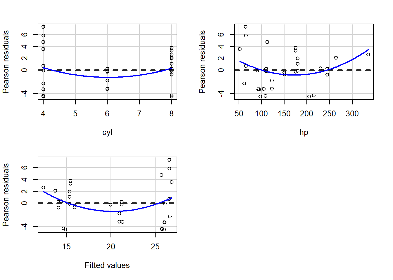
##            Test stat Pr(>|Test stat|)
## cyl           1.2230          0.23151
## hp            2.2362          0.03349 *
## Tukey test    1.9657          0.04933 *
## ---
## Signif. codes:  0 '***' 0.001 '**' 0.01 '*' 0.05 '.' 0.1 ' ' 1
These results allow us to test the following OLS regression assumptions:
- Coefficients are linearly related to the dependent variable.
- Residuals and fitted values are not correlated.
- Population mean of the error term is 0.
- Independent variable and residuals are not correlated with each other.
- No heteroskedasticity in residuals.
Now we will interpret these results.190
In the table above, we see one row for each numeric independent variable in the regression model. Each of these are a lack of fit test for that independent variable. If the p-value is low,191 that means there is evidence for non-linearity, meaning a non-linear relationship between the dependent variable and independent variable. This is something we need to fix in the regression and then re-run it. You have not yet learned much in our course about how to do this. If the p-value is high, that suggests that everything is probably fine.
And then we see a Tukey test result in the final row of the table. This tells us if there is evidence of a relationship between the residuals and the fitted values. One of the OLS regression assumptions is that there is NOT supposed to be a relationship between residuals and fitted values. If this test has a low p-value, there is evidence of some association (relationship) between residuals and fitted values, meaning that you can’t trust the results of your model. If this test’s p-value is high, our model probably doesn’t violate the regression assumption that the residuals are uncorrelated to the fitted values (in other words, the regression is likely trustworthy when it comes to this particular regression assumption).
Example interpretation:
- The
cylp-value is0.23, so there is no evidence to suggest a lack of fit betweenmpgandcylin this regression. - The
hpp-value is very low (less than 0.1), meaning that there’s a more than 90% chance that there’s a lack of fit problem. This is a red flag and we should change how we specify (which variables we put into) the regression model before we trust its results. - The Tukey test p-value is also very low, meaning that our residuals are likely correlated with our fitted values, which is a problem. So we can’t trust this regression result.
The plots that are part of the output are visual representations of what is discussed above, and you can see that all of them are curved (even the cyl one), which displays the non-linearity that the tests in the table show.
You can also see a clear relationship between the residuals and fitted values. You’ll recall that a residual is the difference between the actual and predicted value (fitted value) for a single observation (row) in your dataset. The residuals are supposed to be uncorrelated with the predicted values.192
In all of the plots, the blue line is the computer’s attempt to fit the data. The dotted black line is just a horizontal line for reference. We ideally want the blue line to be flat and right on that black dotted line.
Later in the course, we will practice how to re-specify our regression model to fix any of the problems revealed by the residualPlots() results.
16.2.4.2 Normality of Residuals
Next, let’s test the normality of the residuals, which is another key assumption of OLS regression. There are multiple ways we can do this. One of the most popular ways is to simply look at a Normal Q-Q plot. There are multiple ways to generate this. What I usually do is I run the following command:
plot(reg2)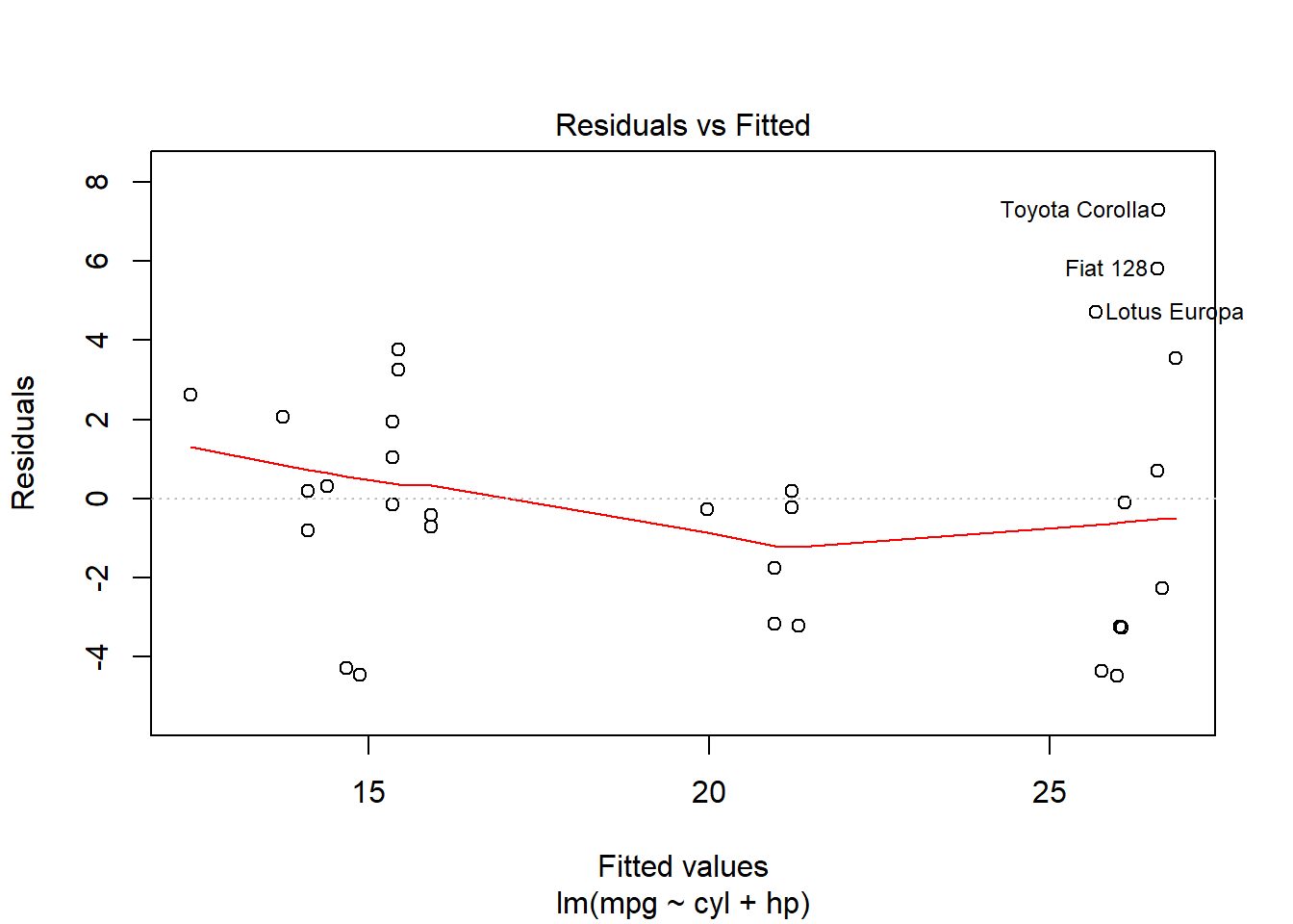
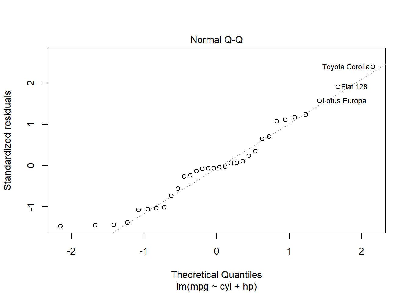
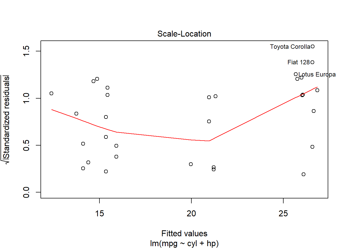
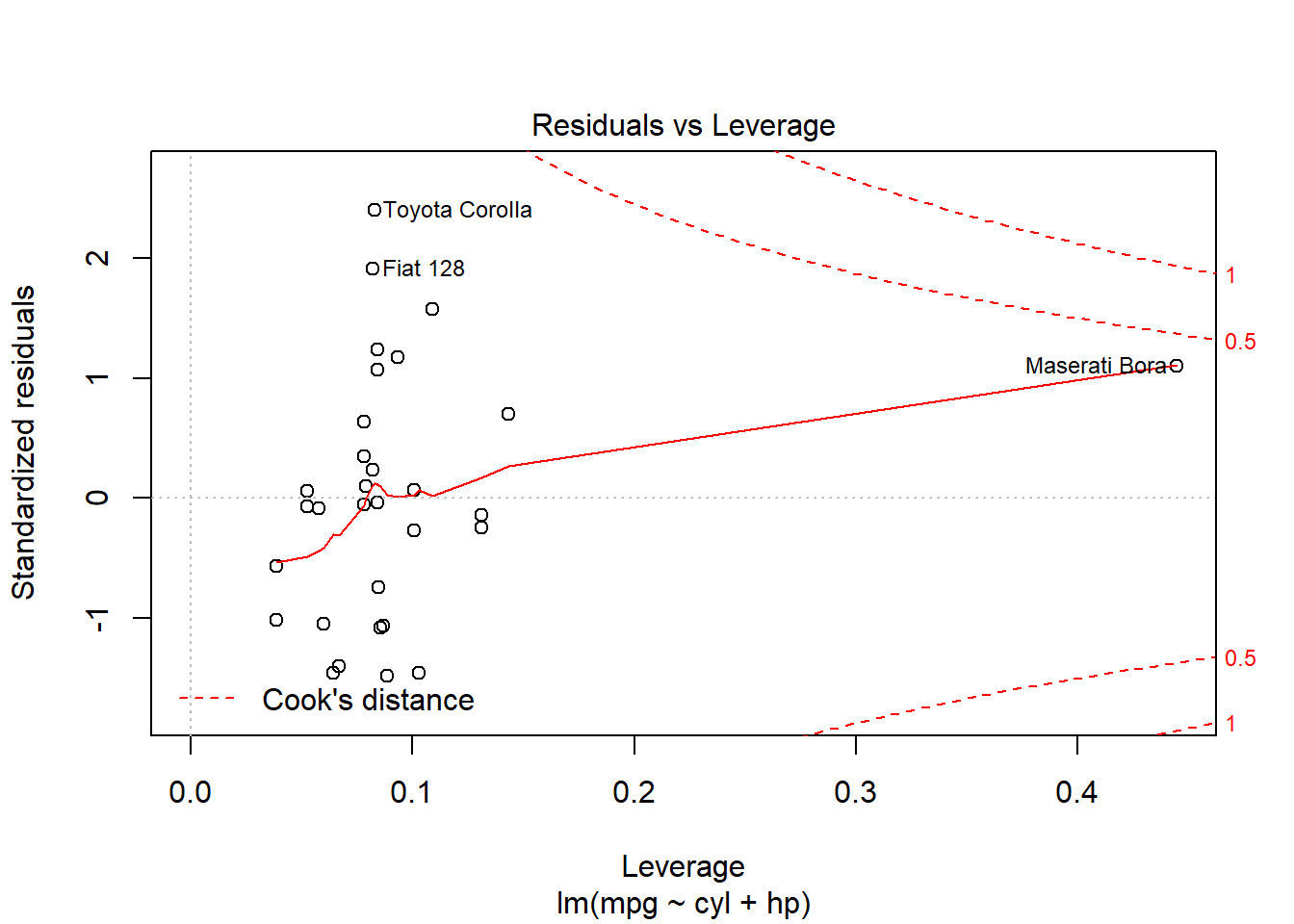
You’ll see that one of the plots above is a Normal Q-Q plot with a dotted line. For now we will only focus on this one. The residuals appear to be somewhat normal, since they are close to the line, but perhaps not as normal as we would like them to be.
The following code will also produce a Normal Q-Q plot:
qqnorm(reg2$residuals)
Another way to test for normality is a simple histogram:
hist(reg2$residuals)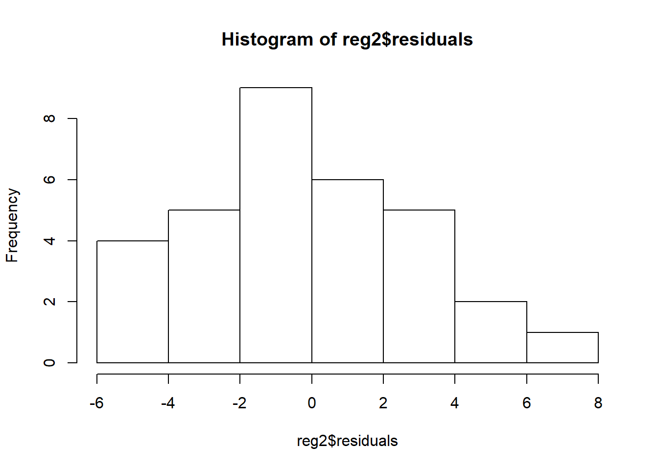
In this, the residuals look fairly normally distributed.
16.2.4.3 Multicollinearity
Finally, we will test the multicollinearity assumption of OLS linear regression. This says that none of the independent variables should be highly correlated with each other. Multicollinearity has nothing to do with the dependent variable or the residuals. It is all about the associations among the independent variables.
The VIF (variance inflation factor) test is the best and most standard way to test for multicollinearity:
library(car)
vif(reg2)
## cyl hp
## 3.256998 3.256998If the numbers you get for any of the independent variables are higher than approximately 4, then you should investigate further. Something I also like to do is make a correlation matrix for the independent variables in the model:
cor(mtcars[c("cyl","hp")])## cyl hp
## cyl 1.0000000 0.8324475
## hp 0.8324475 1.0000000Here we see that our two independent variables actually are pretty highly correlated, so even though the vif test came in under 4, there still may be cause for concern.
When two or more independent variables are highly correlated with each other, the slope estimates are not affected, but the standard errors (confidence intervals) become estimated incorrectly. Therefore, if you want to use your regression model for inference (which is usually what we want to do), you can’t trust the results if you have multicollinearity in your model.
Multicollinearity can be resolved by removing one or more independent variables from the regression model. There are also more advanced ways to resolve multicollinearity while still keeping all variables in the model, but, for now, removing one or more variables should be your strategy of choice. This is also my primary strategy when I encounter multicollinearity, even though I do know some of the other strategies.
16.3 Assignment
In this week’s assignment, you will practice running an OLS linear regression analysis with multiple independent variables as well as all of the diagnostic tests for OLS regression.
16.3.1 Multiple Linear Regression
We’ll start by building a linear regression model.
We’re going to be using a dataset from the car package called GSSvocab. To access this data, please run the following:
library(car)
data("GSSvocab")
Once you do that, you’ll see that the dataset GSSvocab has been added to your environment in RStudio.
In your console, run the command ?GSSvocab. This will pull up some information about this dataset.
Next, I suggest that you just make a copy of the dataset in which any missing values have been removed:
GSSvocab2 <- na.omit(GSSvocab)Now you can use GSSvocab2 as your dataset for the rest of the assignment. You can use a shorter name than GSSvocab2 in the code above, to make it easier to type.
We will be trying to answer the following research question: Are age, gender, and years of education associated with vocabulary?
The names of the four variables you will use are age, gender, educ, and vocab.
Task 1: Identify the independent and dependent variable(s) in this question.
Task 3: Run a linear regression to answer your research question. Remember that your model will have multiple independent variables, unlike last week’s assignment. Please make sure that the regression results table appears in your submitted assignment.
Task 4: Write the equation for the regression results that you got above. Remember that this equation will now have multiple independent variables.
Task 5: Write a single sentence each with the interpretation of the coefficients for age, gender, and educ. (You will write three sentences total).
Task 6: Look at the confidence intervals and p-values for the coefficient estimates for age, gender, and educ. What do each of them suggest about the relationship between each independent variable and the dependent variable in the population at large?
Task 7: How much vocabulary does our regression model predict someone with the following characteristics will have?
18 years old, female, 16 years of education.
Task 8: In your own words, explain what a predicted value is in the context of regression analysis.
Task 9: In your own words, explain what a residual is in the context of regression analysis.
Task 10: In your own words, explain what an actual value is in the context of regression analysis.
Task 11: In your own words, explain what a fitted value is in the context of regression analysis.
16.3.2 OLS Diagnostics
Now you will use the same regression model that you created above, with the GSSvocab data, to test the OLS regression assumptions.
Please start by running the residualPlots() function on the regression model.
Task 12: Are the coefficients linearly related to the dependent variable?
Task 13: Are the residual and fitted values correlated?
Task 14: Are any of the independent variables and residuals correlated with each other?
Task 15: Do any independent variables fail the goodness of fit test?
Task 16: Is there any heteroskedasticity in the residuals?
Task 17: Are the residuals normally distributed?
Task 18: Is there any multicollinearity in the regression model? If so, which variables are causing the problem?
16.3.3 Logistical Tasks
Task 19: Include any questions you have that you wrote down as you read the chapter and did the assignment this week.
Task 20: Please submit your assignment to the online dropbox in D2L as a PDF or HTML file (which you created using RMarkdown193). Please use the same file naming procedure that we used for the previous assignments. Email submission is no longer necessary (but if you have pressing questions, do still send me an email, of course!)
Although it may not be prudent to put too many independent variables, as we’ll see soon.↩︎
Each additional horse?↩︎
Optionally, only if you want, you could read more about the
residualPlots()function and how it works in: Chapter 6, Section 6.2.1 “PLOTTING RESIDUALS” (specifically pp. 288-290) of: Fox, J., & Weisberg, S. (2018). An R companion to applied regression. Sage publications. – The relevant chapter may be available here: https://www.sagepub.com/sites/default/files/upm-binaries/38503_Chapter6.pdf.↩︎For many statistical tests, we use a threshold of p < 0.05 to determine if the test is significant or not. However, for this test of linearity and fit, I recommend that you do not keep a specific threshold in mind. You need to look visually at the plots produced, alongside the p-value for the test result. Then, you can make a fully informed decision about whether to change how you specify the model or not.↩︎
Predicted value and fitted value mean exactly the same thing.↩︎
You can also submit your raw RMarkdown file as well, if you wish↩︎