Chapter 14 ANOVA and Interactions
This chapter is not part of the course HE802 in spring 2021.
- Become acquainted with the basic use and exporting (called “knitting”) of R Markdown files.
Please remember to write down any questions you have as you go through the chapter. Submit these questions along with your assignment.
Possibly useful as you read:
- On a Windows or Linux computer, to open a link in a new browser tab, hold down the
controlkey and then click on the link. - On a Mac computer, to open a link in a new browser tab, hold down the
commandkey and then click on the link.
Announcements and reminders
- You can do this week’s assignment using data of your own (instead of the data provided in the assignment) if you would like and if it is appropriate176 for doing so. Feel free to contact Anshul and Nicole to double-check if your data is a well-suited substitute for the data provided in this or any future assignment. If you are already fairly certain that your own data will be a good substitute, you can go ahead and use it without checking first!
14.1 Answers To Your Questions
Here are some answers to questions I have received over the last week or more that I think might be helpful for everyone to see. You are not required to read these.
14.1.1 R Is Not Working
Many of you have reported that it can be difficult and time consuming to get your R code to run successfully. Many of you have spent a long time trying to fix these problems by looking up what to do, watching videos, etc.
I recommend that you try to fix such issues for 5–15 minutes when they happen, but after that, just ask me what to do. I’m often available to have a phone call or Zoom call and we can quickly resolve the issue.177
14.1.2 Import Excel Data
Here’s how you can import data from Excel into RStudio Cloud.
First, upload your Excel file into your files in the cloud. Make sure the working directory (current folder) is set to the same folder in which your Excel file is. If you haven’t created any new folders, then your file will probably get uploaded to the /cloud/project folder, in which case you don’t need to re-set the working directory.
Next, run the following code:
if (!require(xlsx)) install.packages('xlsx')
library(xlsx)

mydata <- read.xlsx(file="Name Of Your File.xlsx", sheetIndex = 1, header=TRUE)

summary(mydata)
Notes:
- You can change
mydatato whatever you want your dataset to be called in R. This name should show up in RStudio’s Environment tab once you run the command. - The
read.xlsx()function has three arguments in the code above. Let’s go through them:file="Name Of Your File.xlsx"– This tells the computer which Excel file you want it to look at. Change this code so that you replaceName Of Your Filewith the actual name of your file.sheetIndex = 1– This tells the computer to look at the first sheet within the Excel file. If you want it to look at sheet #3, change the1to3in this code.header=TRUE– This tells the computer that the very first row of your Excel file contains variable names, and not raw data.
14.1.3 P-values in T-tests
Sometimes you will be in a situation where you are using different types of t-tests on the same data, and these may give you different results. And even more confusingly, sometimes some may have a p-value of over 0.05 and others will be under. How do we deal with this situation?
In general, there should be one single t-test that is right for your particular situation. I would report the results of that t-test only and explain why you chose that particular t-test. However, if the test result is anyway hovering around p = 0.05, then we have to also consider what this means in plain words. It means that the probability that we’re making an incorrect conclusion is around 5%. If the p-value is 0.051 then the chance we’re making a mistake is 5.1%. And if the p-value is 0.049 then the chance we’re making a mistake is 4.9%. So it’s not actually a big difference in the results between the two t-tests. They’re both telling you approximately the same thing, and we want to report this as accurately as possible in our results. If we were presenting these results, we would want to tell our audience that our p-value is around 5 and so we’re much less certain about this finding than many others which have lower p-values.
14.1.4 Missing data in R
How do we tell R that we want a particular data point to be coded as missing?
We use the built-in NA value. You can use NA as if it is a number. It does not need to be in quotation marks.
Here is an example:
demo1 <- mtcars # make a copy of the mtcars dataset
demo1$cyl[demo1$cyl==8] <- NA # recode 8 as NA for cyl
Above, in the dataset demo1,178 for all observations for which the variable cyl is equal to 8, we have changed those values to NA (missing).
You can run the code above and then run the View() function to see that the change has indeed been made:
View(demo1)
14.2 ANOVA Basics
The entire focus of this week is ANOVA (analysis of variance).
Please read the following resources:
- Sections 2–5 in Analysis of Variance chapter in Online Stat Book – This gets into detail regarding the math behind ANOVA, so you can skim over those parts. You won’t have to do these calculations, but it can be helpful to understand what is going on behind the scenes with the analysis.
One-way ANOVA is used when you have more than two means from independent groups that you want to compare. For example, say you were interested in learning outcomes from 4 different instructional formats. Students were randomly assigned to one of the four formats, and all students then took a test to determine how much they learned. We would use a one-way ANOVA to determine if there are differences between any of the four means.
Why not just compute t-tests comparing each possible set of means? Doing so would increase your likelihood of making a Type I error. For example, if you had 5 groups, that would mean doing \(\frac{k(k-1)}{2} = \frac{5(5-1)}{2} = 10\) independent t-tests. With 10 t-tests with an alpha of .05, there is a 40% chance of observing a statistically significant result. In other words, conducting multiple tests leads to an inflated alpha level.
A one-way ANOVA is an omnibus test that controls the type I error rate. If your overall F-value is statistically significant (p<.05), this indicates that at least two of the group means are different. How do you determine which group means are different from one another? You’ll need to perform post-hoc tests to compare the group means.
14.2.1 Assumptions of ANOVA
ANOVA is part of the general linear model. The assumptions that must be met for One-Way and Factorial ANOVA are similar to those we saw last week:
- Independence of observations. Each participant can only be in one group, and the participants in each group are different.
- The residuals of the dependent variable are normally distributed
- Homogeneity of variances. The variances should be similar across the groups
Before running an ANOVA, you should confirm that your data meets the assumptions of the test.
To test for Homogeneity of Variances:
- Levene’s test
To examine Normality Assumption:
- Plot histograms of the dependent variable for each group/level of your independent variable
- Plot the residuals with a Q-Q plot
- Shapiro-Wilks test (note that when you have large samples (>30-40), this test can be significant even though the data might actually be normally distributed; you should use all of these different pieces of information together to make a determination about normality
Differences between means in an ANOVA are tested with a F-ratio. The F-ratio tests the overall “fit” of the model to the observed data. It is a ratio of explained variability to unexplained variability (error). If the F-ratio exceeds a critical value (dependent on the degrees of freedom in your model), then you know there are significant differences in the means (p<.05).
14.2.2 Post-Hoc Tests and Planned Comparisons for One-Way ANOVA
Post-hoc tests are performed when you do not have any a priori hypotheses regarding which means are different. Post-hoc tests involve conducting pairwise comparisons of all the different combinations of your independent variable. Essentially, it involves conducting multiple t-tests—one for each possible comparison of the groups. But wait… didn’t we agree before not to do this?!
When we conduct multiple statistical tests, we increase the likelihood of committing a Type I error—rejecting the null hypothesis when the null hypothesis is true. Post-hoc tests control for the family wise error rate. Many different post-hoc tests are available that control the overall Type I error rate.
Two common post-hoc tests are the Tukey and Bonferroni tests. These tests are conservative—they control Type I error by adjusting the error rate, but they come at the cost of low statistical power. This means you increase your likelihood of making a Type II error—failing to reject the null hypothesis when there are meaningful differences between groups.
There are many other options for post-hoc tests. We will review how to look at some of them in R.
Planned comparisons are used when you do have a priori hypotheses about the nature of differences across your groups. Typically, this involves comparing two means, so the concern about Type I error rate inflation is not an issue. Planned comparisons involve the use of contrast coefficients, which allow you to “chunk” groups together to compare to another “chunk” of groups (or maybe just one group—for example, if you had three experimental conditions and a control condition, you could use contrasts to compare the three experimental groups together versus the control condition).
14.3 Factorial ANOVA
Please read the following resources:
A factorial ANOVA is used when you have more than one categorical independent variable. If you have two independent variables that each have two levels, this is referred as a 2x2 design. If you had two independent variables, one with two levels and one with three, this would be a 2x3 design.
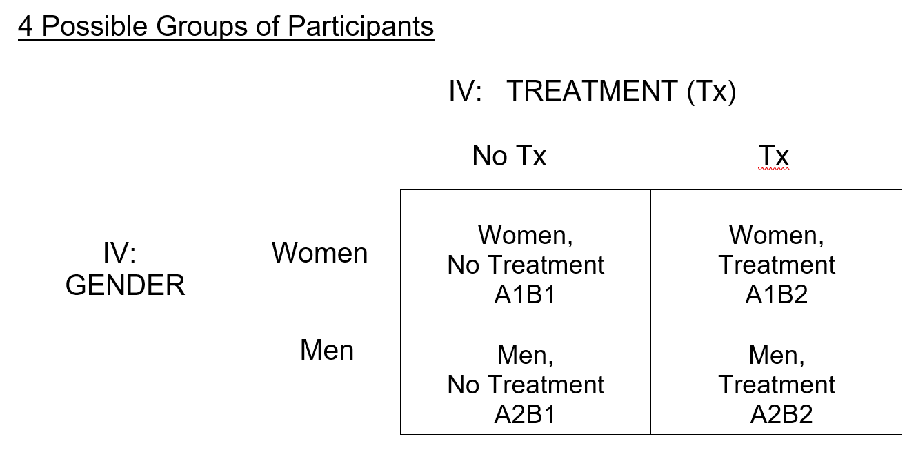
Let’s take the example of a 2x2 ANOVA. A researcher is interested in the effect of an anti-depressant drug on men and women. She randomly assigns a group of 10 men and 10 women to receive either the drug or a placebo (control). She is interested in whether the effect of the drug on depression symptoms is the same for men and women. In other words, she is interested in the interaction of treatment and drug.
Simple 2 x 2 Factorial Design:
- Independent Variable #1 (Factor A): Gender – participants are either male or female
- Independent Variable #2 (Factor B): Treatment – participants either receive the drug or receive a placebo (also called a control condition)
With a factorial design, you can ask the following questions:
- Is there an overall main effect of independent variable #1? – Is there a significant difference in depression between the treatment and no treatment groups?
- Is there an overall main effect of independent variable #2? – Is there a significant difference in depression between men and women?
- Is there an interaction between the two independent variables, such that the effect of one independent variable depends of the level of the other independent variable? – Does the effect of the drug on depression depend on whether participants were male or female?
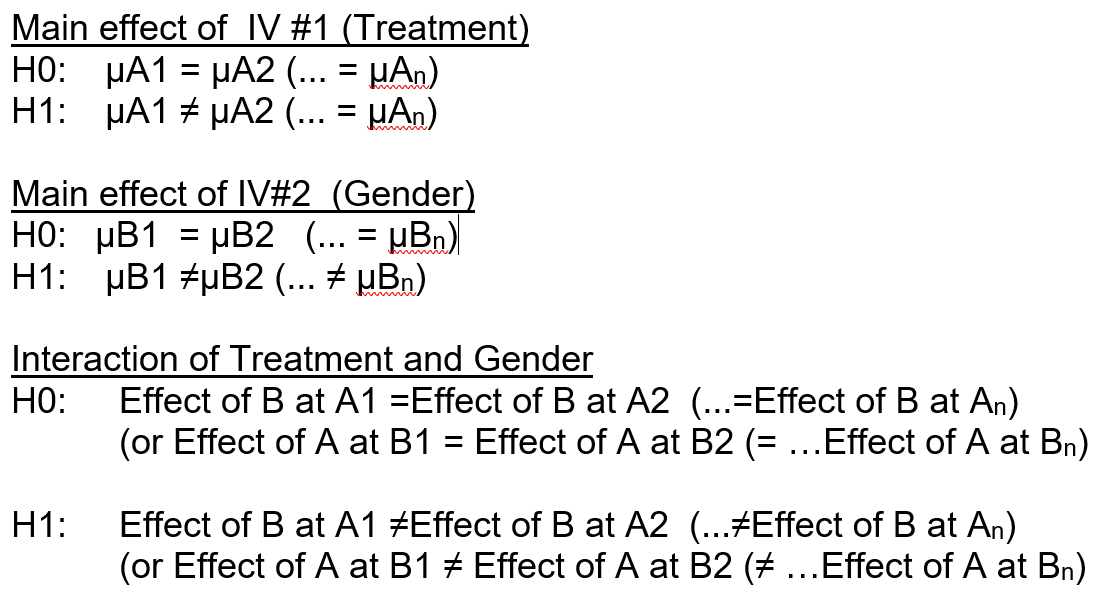
The Null and Research Hypotheses in a Factorial Design, above
When running an ANOVA, the p-values for the main effects and interaction(s) will tell you if there is a significant difference between the groups, or between the different levels of the groups, respectively. If the interaction is significant, you should be cautious in interpreting any significant main effects. This is because although there may be an overall difference between groups on one independent variable, the interaction indicates that the effect of the independent variable on the dependent variable depends on the level of the other independent variable.
14.3.1 Post-Hoc Tests
When you have more than 2 levels of an independent variable and there is a significant main effect or interaction, you will need to conduct post-hoc test or planned comparisons to determine which means are significantly different. If there are only two levels of the independent variable, you can interpret the difference between the two means as significant.
14.4 Repeated Measures and Mixed Design ANOVA
Please read the following resources:
14.4.1 Repeated Measures ANOVA
In some research designs, participants are exposed to several levels of an independent variable and complete the same set of measures on more than one occasion. Repeated Measures designs are used when the same group of individuals participates in all of the different treatment conditions. These designs are sometimes referred to as within subjects designs. Longitudinal studies are also a form of repeated measures.
The strength of within-subjects designs is that person-level variability is controlled for in the analysis. As such, these designs typically require fewer participants. Basically, in a within subjects design, each participant serves as his or her own control.
14.4.2 Mixed-Design ANOVA
Note that “mixed design” ANOVA is not the same thing as a “mixed effects” ANOVA. A “mixed effects” ANOVA (or regression) is a technique that involves modeling the non-independence of repeated measures (or nested) data. For the purposes of this class, we will only focus on mixed-design ANOVAs.
In a mixed design ANOVA, there is at least one between-subjects independent variable, and at least one within subjects variable. Essentially, it is the combination of a factorial ANOVA and a repeated measures ANOVA. Your between subject factor(s) will be the variable that groups your participants—for example, intervention versus control, men v women, placebo v experimental drug, etc. Your within subjects factor(s) will be the variable or variables on which you take multiple measurement—for example, pre and post measurements, measures of symptoms at 4 different doses of a drug, etc.
This is a popular study design because it combines the strengths of both between subjects and within subjects designs.
Assumptions of the Mixed Design ANOVA:
- Homogeneity of variances
- Sphericity
Interpreting the Results of a Mixed Design ANOVA: When interpreting the results of a mixed design ANOVA, you follow the same rules you did when interpreting between and within subjects designs:
- For between subjects main effects: If there are 2 levels, a significant F statistic indicates the means of the two groups are significantly different. If you have three or more levels, you will need to do post-hoc comparisons to identity which pair or pairs of means are significantly different.
- For within subjects effects: If there are 2 levels, a significant F statistic indicates the means of the two conditions (or time points) are significantly different. If you have three or more levels, you will need to do post-hoc comparisons to identity which pair or pairs of means are significantly different.
- For the interaction of between and within subjects variables: The pattern of means is different across conditions. In other words, the effect of one independent variable depends on the level of the other independent variable. You may need to do simple effects or contrasts to unpack the nature of the interaction (depending on how many conditions there are for your IVs).
14.5 Covariates and ANCOVA
Please read the following:
In the context of an ANOVA, a covariate is a continuous independent variable. Typically, covariates are variables that you want to control for in an analysis. An Analysis of Covariance (ANCOVA) is an ANOVA that includes a covariate. The variability associated with covariate is controlled for, and then the ANOVA is conducted (R will do all of this behind the scenes).
Controlling for covariates increases your precision in detecting treatment effects. The variability associated with the covariate is “noise” in your dependent variable. By including the covariate, you decrease the “noise” and improve your ability to detect the “true” effect of your manipulation.
An example: You are interested in the impact of an intervention on the empathy of doctors. Doctors are randomized to either a control condition or an intervention condition. Empathy is measured before, immediately after, and 6 months after the intervention takes place. Although there are a number of ways you could analyze this data, one way would be to treat pre-test empathy scores as a covariate in the analysis. You would then examine differences in empathy at the two remaining time points, controlling of level of empathy before the intervention.
Another example: You are comparing men and women’s performance on the MCAT. An analysis of demographic differences between the two groups reveals that the men are significantly older than the women. You would then include age as a covariate in any of the analyses you conduct to account for the differences in your two groups.
Another term you might hear is confounder. A variable is considered a confounder if it is associated with both your independent and dependent variable. Confounders can bias your results and also need to be controlled for in your analyses.
Determining whether to include a covariate in your analysis:
- Based on the scientific literature, is there a variable (or set of variables) that is generally known to be associated with your outcome, and have you measured it as part of your study? (This means you have to give consideration to covariates at the design state of research—not after the fact!)
- Is the variable correlated with your outcome variable? If the variable is not associated with your outcome, it doesn’t make sense to include it in your analysis.
14.6 Conducting ANOVA in R
These resources will be useful as you do this week’s assignment:
- ANOVA – A good starting point.
- One-Way ANOVA Test in R
- Two-Way ANOVA Test in R
- R ANOVA Tutorial: One way & Two way (with Examples)
- How to Calculate ANOVA Using R
- Repeated Measures ANOVA in R – This one is likely to be helpful on the final portion of your assignment this week.179
14.7 Assignment
This week, you are required to use an RMarkdown document to do your assignment. By the end of this week, you should be fully comfortable with making an RMarkdown document and exporting it as a PDF and/or HTML file.180
14.7.1 Management Study
A random sample of non-management employees was taken at a southeastern area community hospital. Using non-self report data collected by the hospital, we have a measure of each person’s productivity, in person hours per/week. We also have information regarding the management style of each person’s supervisor, broken down into 4 categories: Direct Management, Collective Responsibility, Strict Hierarchy, and non-hierarchical working groups. For the purpose of this assignment, we will ignore the non-random sampling to levels of the independent variable, and the potential non-independence in the data. The dataset, called management style.csv, is available here.
You may need to do the following to convert certain variables from numeric to categorical:
DataSet$NewVariable <- as.factor(DataSet$OldVariable)Task 1: Conduct the appropriate ANOVA analysis to examine mean differences across the four conditions. Report the F, degrees of freedom, and p-value for the main effect of condition.
Task 2: Produce a box plot181 of the means on productivity for each condition.
Task 3: Does the data violate the assumption of homogeneity of variances? Report the appropriate test statistic and its significance level.
Task 4: Produce a set of pairwise comparisons using the Tukey test. Report which pairs of means are significant at the p<.05 level.
Task 5: Write a brief paragraph that summarizes your findings.
Task 6: Given your findings, are there any further analyses or contrasts you think might be appropriate for the data? Why?
14.7.2 Identify Effect Types
Task 7: The six figures below show the population means for six experiments. For each one, indicate whether an A effect, a B effect, and/or an AxB interaction is present (in some figures, more than one of these effects are present).

14.7.3 Cholesterol Study
This exercise will use the freely available cholesterol dataset.182 You can download it from here. This dataset is in SPSS format. You can use the following code to load it into R:
if (!require(foreign)) install.packages('foreign')## Loading required package: foreignlibrary(foreign)
cholesterol <- read.spss("Cholesterol.sav", to.data.frame = TRUE)## re-encoding from UTF-8The study tested whether cholesterol was reduced after using a certain brand of margarine as part of a low fat, low cholesterol diet. The subjects consumed on average 2.31g of the active ingredient, stanol easter, a day. This data set contains information on 18 people using margarine to reduce cholesterol over three time points. Participants were randomly assigned to use one of two margarines (Margarine A or B). For the purposes of this question, interpret all findings that are p <.10 as significant.
Information about the data:
| Variable name | Variable | Data type |
|---|---|---|
| ID | Participant number | |
| Before | Cholesterol before the diet (mmol/L) | Scale |
| After4weeks | Cholesterol after 4 weeks on the diet (mmol/L) | Scale |
| After8weeks | Cholesterol after 8 weeks on the diet (mmol/L) | Scale |
| Margarine | Margarine type A or B | Binary |
You may need to reshape the data from wide to long, as described here:
The resource above is also a reasonable guide for conducting the rest of this portion of the assignment.
Task 8: Conduct a mixed-design ANOVA to answer the following questions:
- Is there a main effect of time on cholesterol?
- Is there a main effect of margarine on cholesterol?
- Is there an interaction between time and the type of margarine?
Also show the following work:
Task 9: Check that the data meets the assumptions of mixed ANOVA (e.g., sphericity)
Task 11: Conduct post-hoc tests, as appropriate
Task 12: Plot the main effects and the interaction
Task 13: Write a short paragraph summarizing and interpreting your results. Include or refer to any tables or figures that are useful in understanding your findings.
14.7.4 Logistical Tasks
Task 14: Include any questions you have that you wrote down as you read the chapter and did the assignment this week.
Task 15: Sometime between February 10–23, you are required to complete a mandatory oral exam on Zoom. Please e-mail me with 2–3 times (lasting at least 1 hour, but 1.5 hours might be even better) when you can meet to do this.
Here is some information about the oral exam:
- Less work will be assigned during the week of February 10, so that you have time to review what we have done so far.184
- For example, you could spend the week of February 10 studying and then have your exam at the end of that week (February 13 or 14, for example). Or you could have the exam during the week of February 17.
- During the exam, I will ask you questions and you will have to answer them. The content will be based on what we have covered in class so far. You may also need to demonstrate skills in R and RMarkdown.
- If you get a grade on the oral exam that you are not satisfied with, you can re-take the oral exam.
Task 16: Please submit your assignment to the online dropbox in D2L as a PDF or HTML file (which you created using RMarkdown185). Please use the same file naming procedure that we used for the previous assignments.
Task 17: Please submit your assignment to me by email.
For example: Your data should be quantitative in nature and contain variables within it that can be analyzed using descriptive statistics, visualizations, t-tests, and similar analysis strategies.↩︎
You can also tell me in advance if you already know when during the week you’ll be working on our course. I can try to be available at that time, in case you need any assistance.↩︎
demo1is just a copy of the datasetmtcarsthat I decided to make for this demonstration.↩︎This resource was added late, on February 10, 2020.↩︎
I encourage you to let me know about any issues you encounter in this process so that we can fix them.↩︎
This accidentally and incorrectly said “box plot” initially. It was corrected on February 10 2020.↩︎
From www.statstutor.ac.uk↩︎
This resource was added late, on Feb 10 2020.↩︎
If you were part of the Masters program in Health Professions Education with us at MGHIHP, you’ll recall that we advocate for spaced learning to be built into any learning curriculum. These oral exams are an attempt to do that. I’ll of course welcome any feedback.↩︎
You can also submit your raw RMarkdown file as well, if you wish↩︎