Chapter 11 Mar 29–Apr 4: Logistic Regression
This chapter is now ready for use by HE802 students in spring 2021.
This week, our goals are to…
Compare linear and logistic regression.
Practice creating and interpreting the results of a logistic regression model.
Optional: Practice testing selected assumptions of logistic regression using diagnostic tests.
Announcements and reminders:
This chapter contains a combination of required and optional content and skills for you to learn. I recommend that you look at the assignment at the end of the chapter before you start this week’s work, so that you have a sense for which skills are required and optional.
If you have not done so already, please e-mail Nicole and Anshul to schedule your Oral Exam #2. The deadline for doing Oral Exam #2 is April 2 2021.
This week, we will have group work sessions on Wednesday and Friday at 5:00 p.m. Boston time, in addition to any meetings that you schedule with us separately. You should already have received e-mail calendar invitations from Nicole for these sessions. Note that these sessions can be treated as office hours for the course, during which you can ask any questions you might have.
11.1 Logistic regression
So far, we have studied OLS linear regression, in which the dependent variable is a continuous numeric variable. But what if your data and research question require you to have a categorical dependent variable? When this is the case, you have to use some sort of classification technique.142 Logistic regression is the typical initial technique that you should try first when you have a categorical dependent variable and when you are interested in investigating the relationship between the probability of that dependent variable and one or more independent variables.
In this chapter, we will only learn about binary logistic regression, in which the dependent variable can only have two levels (for example, good or bad, 1 or 0, functional or non-functional, admit or not admit). In other words, the dependent variable must be a dummy variable.
11.1.1 Linear compared to logistic regression
Let’s look at some of the differences and similarities between linear regression and logistic regression.
Consider the following scenarios:
| Question (casual wording) | Question (more precise wording) | Dependent variable | Levels of dependent variable | Independent variables | Regression model used to answer question |
|---|---|---|---|---|---|
| Are students who study a lot more likely to pass the test than students who do not study as much? | In a sample of students, is likelihood of passing a test associated with hours spent studying for the test, controlling for demographic characteristics? | Test result | pass, fail | hours spent studying, gender, socioeconomic status, age | Logistic regression |
| Are people who work out a lot more fit than people who don’t? | In a sample of athletes, is the time it takes to run one mile associated with number of visits to the gym per week, controlling for demographic characteristics? | Time in seconds required to run one mile | Any fractional or whole number | number of days per week going to the gym, gender, socioeconomic status, age | Linear regression |
As we see in the two scenarios above, we choose our regression model depending on the dependent variable. A dependent variable that is not numeric—such as passing or failing a test—requires logistic regression. A dependent variable that can be measured as a whole or fractional number143—such as time required to run a mile—can be analyzed using linear regression.
Keeping these examples and types of dependent variables in mind, what are we trying to predict in linear regression and logistic regression?
With linear regression, we create a regression model (which can be described by an equation) that tells us the relationship between the dependent variable and each independent variable. We then use this equation to calculate predicted values of the dependent variable for each observation (data point). Our goal is for these predicted values to be as close to the real values of the dependent variable as possible. Our primary goodness-of-fit test is the R-squared statistic, which tells us how close the predicted values are to the real values of the dependent variable.
In logistic regression, we also create a regression equation that tells us the relationship between the dependent variable and each independent variable. We then use this equation to calculate predicted probabilities that each observation (data point) falls into one category of the dependent variable rather than another. The goal is to accurately predict which category each observation is in. There are multiple possible goodness-of-fit tests for logistic regression, which examine how well A) our predictions about the category of the dependent variable into which each observation falls matches with B) the reality of the category into which each observation falls.
How do we interpret the regression equation?
In linear regression, each estimated regression coefficient tells us the relationship between one independent variable and the dependent variable. The coefficient tells us the predicted change in the dependent variable for each one-unit increase in the independent variable (or the predicted difference in the dependent variable for a dummy variable, compared to the reference category).
In logistic regression, each estimated regression coefficient also tells us the relationship between one independent variable and the dependent variable. However, the coefficient is telling us the multiplicative relationship between the independent and dependent variable. We will typically prefer to look at the coefficient in its odds ratio form, which we will learn about later in this chapter. The logistic regression is predicting that for every one unit increase in the independent variable, the predicted likelihood of an observation being in the 1 category (rather than the 0 category) of the dependent variable is multiplied by the coefficient. Note that we use the same magic words as always to interpret our results, even for logistic regression.
How do we know the extent to which the relationships predicted in the regression results might also be true in the population from which the sample was drawn?
Inference works the same way for linear and logistic regressions. You should look at the confidence intervals and p-values for each estimated coefficient. The meaning of the p-value is the same in both cases. It is the result of a hypothesis test regarding the relationship between the dependent variable and independent variable.
Of course, as is the case with linear regression, all of the assumptions of logistic regression need to be met before you can consider your results to be trustworthy. We will look at some of the key logistic regression assumptions in this chapter.
11.1.2 Optional videos and resources
The videos and resources in this section are optional to watch or read. The videos contain some introductory material that demonstrates how logistic regression works and how the computer fits a regression model using maximum likelihood estimation. The additional readings explain some of the more technical details and theory related to logistic regression, more than you are required to know in order to use logistic regression effectively and responsibly.
The following StatQuest video from Josh Starmer is a good introduction to the concept of logistic regression:144
The video above can be viewed externally at https://www.youtube.com/watch?v=yIYKR4sgzI8.
And the following video—also a StatQuest video with Josh Starmer—discusses the basic method used in maximum likelihood estimation, which is the procedure that the computer uses to fit a logistic regression model to our data:145
The video above can be viewed externally at https://www.youtube.com/watch?v=XepXtl9YKwc.
Some of the concepts demonstrated and discussed in the optional videos above will be used throughout this chapter.
If you want to learn more about the technical details and theory related to logistic regression models, you can have a look at the following resources. Keep in mind that it is not required for you to read these.
Optional additional information about logistic regression:
Chapter 16, “Logit Regression” in: Jenkins-Smith, Hank; et al. Public Administration: 4th Edition With Applications in R. https://bookdown.org/josiesmith/qrmbook/.
Chapter 4,“Logistic regression” in: Portugués, E.G. (2017). Lab notes for Statistics for Social Sciences II: Multivariate Techniques. https://bookdown.org/egarpor/SSS2-UC3M/.
11.1.3 Selected logistic regression math
This section contains details that are optional (not required) to read and learn. Below, we look at some basic details of how we can fit a regression model to a binary dependent variable. If you do choose to read this section, as you read it, keep in mind that this is an abbreviated explanation of what we are doing in logistic regression, just so what you have some intuition for it as you run logistic regressions and interpret the results.
In linear regression, we fit a linear equation to our data:
\(\hat{y}=b_1x_1+b_2x_2+...+b_0\)
For logistic regression, it does not make sense to fit a linear equation to our data, because the dependent variable can only have two possible values, 0 and 1. In logistic regression, instead of trying to predict the value of the dependent variable, we are trying to predict the probability that the dependent variable has a value of 1 instead of 0.
We write the probability of the dependent variable—called \(y\)—being equal to 1 like this:146
\(P(y = 1)\)
And we can write the odds of the dependent variable being equal to 1 like this:147
\(\frac{P(y = 1)}{1-P(y = 1)}\)
If we take the natural logarithm of the odds above, we get what we call the logit of \(y\):148
\(logit(y) = log_e(\frac{P(y = 1)}{1-P(y = 1)})\)
\(logit(y)\) can vary from a very low number to a very high number and it can vary linearly with our independent variables. So, when we do logistic regression, we fit the following model:
\(\hat{logit(y)} = b_1x_1+b_2x_2+...+b_0\)
The right side of the equation above should look familiar because it is the same as our linear equation that we used for linear regression. The predicted values from our logistic regression equation above will give us predicted values of \(logit(y)\).
Once we do that, we have to interpret the results so that we can learn about how the probability of the dependent variable being equal to 1 is associated with our independent variables. T do this, we exponentiate \(logit(y)\). This means that we raise the mathematical constant \(e\) to the power of \(logit(y)\). We then replace \(logit(y)\) with \(b_1x_1+b_2x_2+...+b_0\).
Here is that process:149
\(\text{odds that y is 1} = e^{logit(y)} = e^{b_1x_1+b_2x_2+...+b_0}\)
For every one unit increase in one of the \(x\) variables, the odds that \(y\) is 1 will also increase or decrease (depending on whether the \(b\) coefficient of that \(x\) variable is positive or negative).
The concepts above are a summary of how we can transform our data to find out the relationship between the odds of \(y\) being 1 and our independent variables or interest. The rest of this chapter focuses on how to apply logistic regression, interpret its results, and determine the extent to which we can trust a logistic regression model.
11.1.4 Model specification for logistic regression
The guidelines for model specification—meaning the decision of which independent variables to include in the model and how to transform and/or interact them—are very similar for linear and logistic regression. In general, we can include transformed independent variables, interaction terms, dummy variables, and continuous numeric variables in any combinations that we wish, as long as doing so will appropriately help us answer our question of interest.
11.2 Logistic regression in R
We will learn about logistic regression by going through an example together in R. Don’t forget that logistic regression is a special type of regression we use when our dependent variable has only two categories which are not numeric.
Here are the details of the example we will go through:
Question of interest: What is the relationship between diabetes status and BMI,150 age, gender, and home ownership status in Americans during the years 2009–2012?
Dependent variable: Diabetes status. This dummy variable will be coded as 1 for people who have been diagnosed with diabetes and 0 for people who have not.
Independent variables: BMI, age, gender, home ownership status.
Dataset: For this example we will use a dataset called NHANES (American National Health and Nutrition Examination surveys) which is conducted by the US National Center for Health Statistics. This data is built into R and therefore convenient for us to use.
Unit of observation: a person living in the United States of America who has been surveyed during the years 2009–2012.
11.2.1 Load and prepare data
First, we will load and prepare our data to be used for analysis. Most of this procedure involves skills that we have already learned about in this textbook. Therefore, not much explanation will be provided as we load and prepare the data.
Our data comes from the NHANES package, which we will install and load with the following code:
if (!require(NHANES)) install.packages('NHANES')
library(NHANES)
Next, we will run the data(...) function to load the NHANES data into R:
data(NHANES)After running the command above, NHANES will be listed as a dataset in our Environment tab in RStudio. You can run the command ?NHANES on your own computer to read about this dataset.
Next, we will make a copy of NHANES called df1, which we will use in the rest of this chapter:
df1 <- NHANESNow that our dataset—called df1—is loaded, we can explore our data a bit.
Here are the dimensions of df1:
dim(df1)## [1] 10000 76df1 has 10,000 observations and 76 variables.
Here, we subset only the variables we plan to use and then again check the dimensions of our dataset:
df1 <- df1[c("Diabetes","Gender","Age","BMI","Poverty","HomeOwn")]
dim(df1)
## [1] 10000 6Now we have 10,000 observations and just six variables!
Let’s explore these six variables:
summary(df1)## Diabetes Gender Age BMI Poverty
## No :9098 female:5020 Min. : 0.00 Min. :12.88 Min. :0.000
## Yes : 760 male :4980 1st Qu.:17.00 1st Qu.:21.58 1st Qu.:1.240
## NA's: 142 Median :36.00 Median :25.98 Median :2.700
## Mean :36.74 Mean :26.66 Mean :2.802
## 3rd Qu.:54.00 3rd Qu.:30.89 3rd Qu.:4.710
## Max. :80.00 Max. :81.25 Max. :5.000
## NA's :366 NA's :726
## HomeOwn
## Own :6425
## Rent :3287
## Other: 225
## NA's : 63
##
##
## It is important to note that many of the variables above have missing data. You can see this in the NA's portion of each variable’s summary. For example, out of the 10,000 rows in our dataset, 366 of these rows (observations) are missing a BMI value. You can pause for a moment to make other observations about these variables before continuing.
We want to remove any observations with missing data, so we run the code below:
df1 <- na.omit(df1)Now we have a clean version of df1 with no missing values for our variables of interest. In the code above, we used the na.omit(...) function with df1—our dataset—as the only argument. We then over-wrote our previous version of df1 with the new version, by putting df1 on the left side of the <- operator.
Let’s inspect the dimensions of the latest version of our dataset df1:
dim(df1)## [1] 8931 6Now we see that we have 8,931 observations remaining—all of which have complete data—that we will use in our analysis.
The next step is to prepare any variables that are not already ready for analysis. In this example, this means converting our categorical variables—diabetes status, gender, and homeownership status—into dummy variables.
Like we have done before, we will use the fastDummies package to accomplish this conversion of variables:
if (!require(fastDummies)) install.packages('fastDummies')
library(fastDummies)

df1 <- dummy_cols(df1,select_columns = c("Diabetes","Gender","HomeOwn"))
We now have the appropriate dummy variables within our dataset df1. You can run the View(df1) command on your own computer to see this.
Here is a list of all our variables:
names(df1)## [1] "Diabetes" "Gender" "Age" "BMI"
## [5] "Poverty" "HomeOwn" "Diabetes_No" "Diabetes_Yes"
## [9] "Gender_female" "Gender_male" "HomeOwn_Own" "HomeOwn_Rent"
## [13] "HomeOwn_Other"Among the list of variables above, there are some variables that we will no longer need to use and others that we will be using. Below is a list of the variables that we will be using as we continue this example.
Diabetes_Yes– This is our dependent variable. It is a dummy variable that we created with 1 coded as yes diabetes and 0 coded as no diabetes.BMI– This is a continuous numeric variable that we did not modify at all from the original dataset.Age– This is also a continuous numeric variable that we did not modify at all from the original dataset.Gender_female– This is a dummy variable that we created with one coded as female and 0 coded as male. We will include this dummy variable in any analysis we do. The reference category for this dummy variable is males, meaning that regression estimates will give us a result for females compared to males.HomeOwn_RentandHomeOwn_Other– These are dummy variables that we created based on the original categorical variable HomeOwn. We will include both of these dummy variables in any analysis we do. The reference category for these dummy variables is people who own their own homes. In regression estimates, theHomeOwn_Rentvariable will compare Americans who rent their homes to those in the reference category who own their homes. In regression estimates, theHomeOwn_Othervariable will compare Americans who fall into theOtherhome ownership category to those in the reference category who own their homes.
You may have noticed that we have not yet mentioned the Poverty variable. We are keeping this in our dataset for future use in this chapter.
11.2.2 Descriptive visualizations and statistics
Now that our data is ready for analysis, let’s start by descriptively visualizing and breaking down our data.
We start with a scatterplot which plots our dependent variable—Diabetes_Yes—against one of our independent variables, BMI:
plot(df1$BMI, df1$Diabetes_Yes)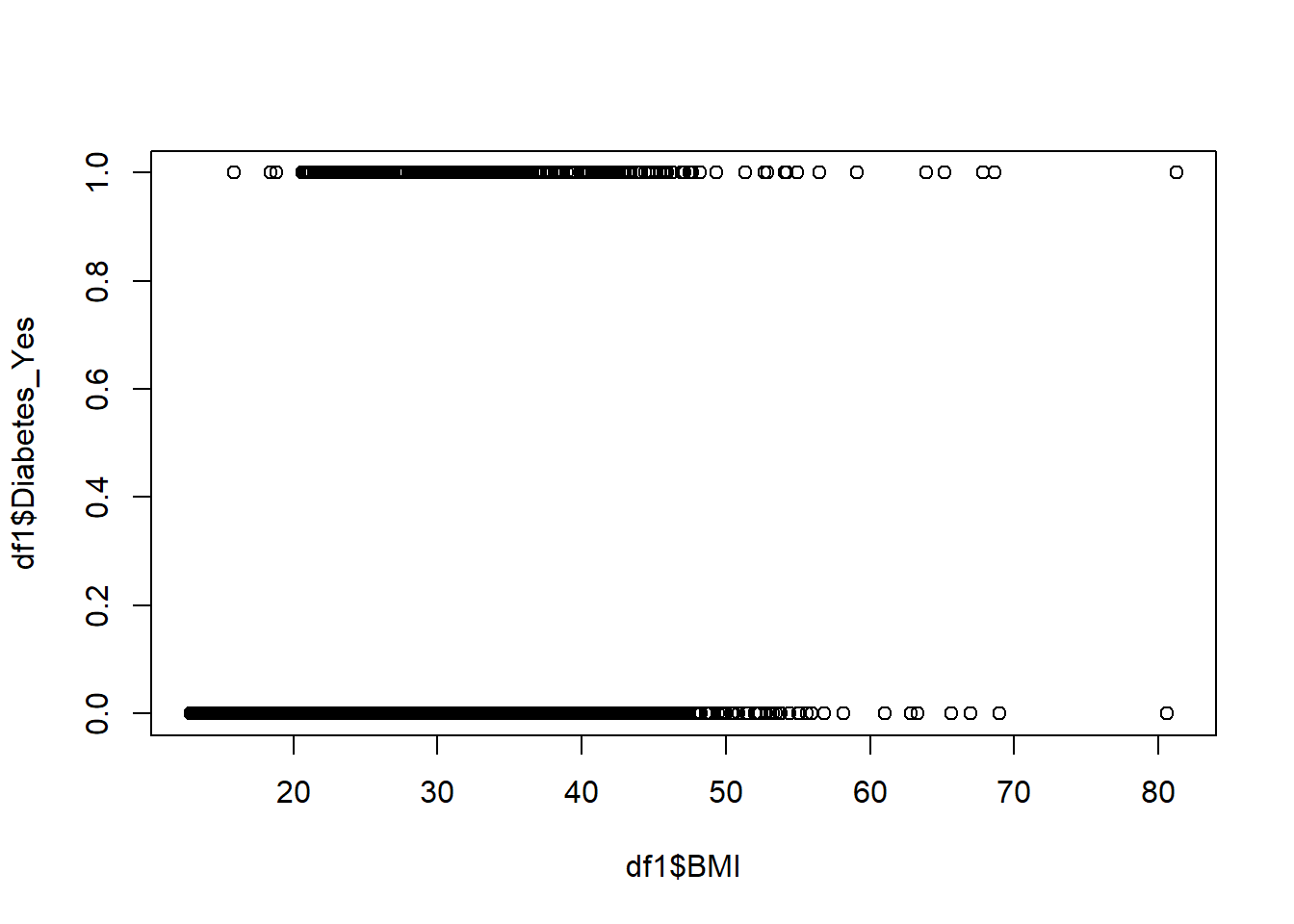
Before this chapter in our textbook, we had always analyzed dependent variables that were continuous numerical variables. In those situations, when we made a scatterplot with a continuous numeric dependent variable on the vertical axis, we could off and see some type of trend between the dependent variable and the independent variable on the horizontal axis. Now, in this chapter, we have a binary dependent variable. The only possible values of our dependent variable are zero, meaning a person has diabetes; or 1, meaning a person does not have diabetes. As you can see in the plot above, it is very difficult to visually determine if there is any relationship between diabetes status and BMI.
Let’s look at another scatterplot, this time diabetes status against age:
plot(df1$Age, df1$Diabetes_Yes)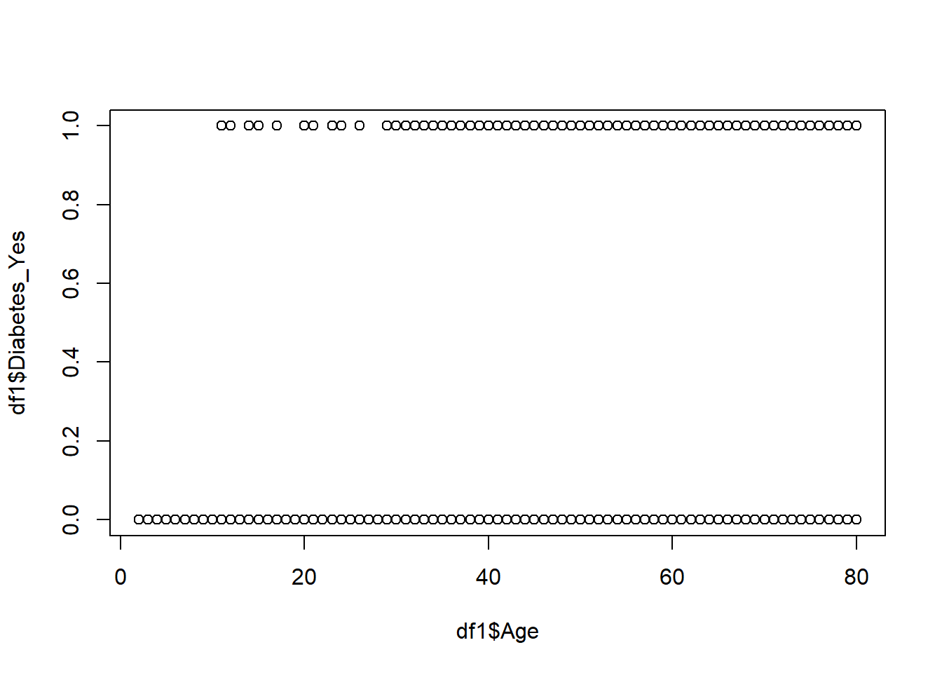
In the plot above, it is still pretty hard to visually determine if there is any relationship between diabetes status and age. However, it appears that all of the people who have diabetes are older than some people who do not have diabetes. More specifically: people between ages 0 and 30 years old visually appear to be more likely to not have diabetes than to have it. And then for ages above 30 years old, we cannot really tell from this scatterplot.
We can also make some two-way tables to explore descriptive relationships between diabetes status and our categorical independent variables.
We begin with a two-way table of diabetes status and gender, below:
with(df1, table(Diabetes_Yes, Gender_female))## Gender_female
## Diabetes_Yes 0 1
## 0 4086 4156
## 1 371 318We can also make a two-way table of diabetes status and home ownership status:
with(df1, table(HomeOwn, Diabetes_Yes))## Diabetes_Yes
## HomeOwn 0 1
## Own 5339 480
## Rent 2718 189
## Other 185 20It is difficult to tell from these tables these two way tables if diabetes status is associated with gender or home ownership status. But that’s okay, because logistic regression is going to come to the rescue.
11.2.3 Visualize logistic regression
Even though it is difficult to do, we are now going to try to visualize what exactly logistic regression is helping us do as we analyze our data and try to answer our question of interest.
Below, we make a simple logistic regression model with diabetes status as the dependent variable and BMI as the only independent variable:
logit.sim <- glm(Diabetes_Yes ~ BMI, data = df1, family = "binomial")Here is what we asked the computer to do with the code above:
logit.sim– Save our regression model as the namelogit.sim- glm(…) – We want to make a regression model that falls into the class of regression models called generalized linear models.
Diabetes_Yes ~ BMI–Diabetes_Yesis the dependent variable andBMIis our only independent variable. A~symbol separates the dependent variable from any independent variables (just one in this case), like in other regression models we have made.data = df1– The variables we want to include in our regression model come from the dataset calleddf1.family = "binomial"– The specific type of regression we want to do is logistic regression. The"binomial"argument here tells the computer that we want logistic regression.
For now, we will not look at a regression table or attempt to numerically interpret the logistic regression model that we just made. Instead, we will visualize our logistic regression results by plotting them on the same scatterplot that we looked at earlier with diabetes status and BMI. To do this, we will have to write some additional code. It is not necessary for you to learn this entire process. The key is to understand what is happening in the scatterplot at the end of this process.
The first step is to create a range of values that we will plug into our regression equation to calculate predicted values:
BMIrange = seq(min(df1$BMI),max(df1$BMI),0.01)Here is what the code above did:
BMIrange– Create a new column of data calledBMIrange. This column of data is not associated with any dataset. It exists in R on its own.- seq(…) – Make a new column of data using the
seq(...)function. min(df1$BMI)– The new column of data will start at the minimum value of the variableBMIwithin our datasetdf1.max(df1$BMI)– The new column of data will end at the maximum value of the variableBMIwithin our datasetdf1.0.01– The new column of data will contain values that increase in increments of 0.01.
Once again, it is not necessary for you to understand the code above. At the same time, I don’t want to hide the entire process from you, in case you do want to run it yourself on your own computer. Above, you would change BMI to the name of your own variable and you would change df1 to the name of your own dataset; you could leave the rest as it is above.
Next, we calculate predicted values of our simple logistic regression model called logit.sim:
logit.sim.prob <- predict(logit.sim, list(BMI = BMIrange), type = "response")Here is what the code above did:
logit.sim.prob– Create a new column of data calledlogit.sim.prob. This column of data will contain predicted probabilities (from the regression modellogit.sim) for each value within the data columnBMIrange.predict(...)– Calculate predicted values from a regression model.logit.sim– Calculate predicted values from the saved logistic regression model calledlogit.sim. This is where the regression equation is stored.list(BMI = BMIrange)– These are the values that will be plugged into the stored regression equation. We plug the values saved inBMIrangein place of theBMIvariable in the regression modellogit.sim.type = "response"– We want our predicted values to be given to us in terms of predictedprobabilities. The"response"argument says that we want predicted probabilities.
Once again, it is not necessary for you to understand the code above. I am just including it here so that it is transparently available to you in case you do want to use it yourself.
Finally, we are ready to recreate our plot of diabetes status against BMI. This time, we also add a regression curve of predicted probabilities.
The following two lines of code give us the scatterplot with our regression curve:
plot(df1$BMI, df1$Diabetes_Yes)
lines(BMIrange, logit.sim.prob)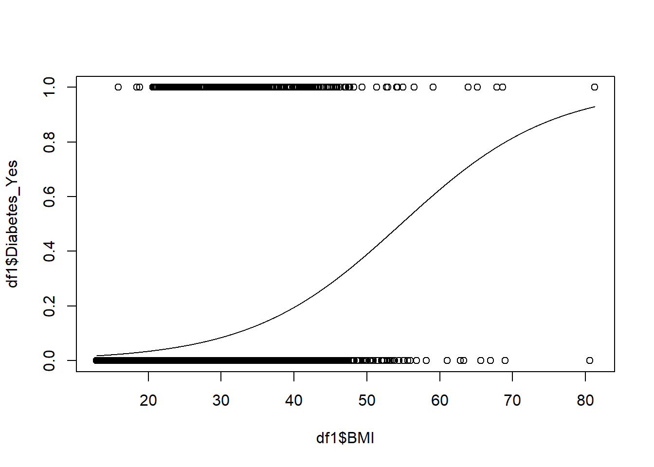
In the two lines of code we used to generate the plot above, here is what we did:
plot(df1$BMI, df1$Diabetes_Yes)– Create a scatterplot with diabetes status on the vertical axis and BMI on the horizontal axis. This is the same way we have always made scatterplots.lines(BMIrange, logit.sim.prob)– Add a line to the already-created scatterplot, with the predicted probability of somebody having diabetes on the vertical axis and BMI on the horizontal axis.
It is not necessary for you to understand the code above.
We have finally reached the important part. Let’s carefully go through the plot above.
We plotted
Diabetes_Yeson the vertical axis andBMIon the horizontal axis, just like we did before, when we were just exploring the data visually.We now have a regression curve in the scatterplot. This curve shows us the results of a logistic regression model. This curve shows the predicted probability of a person having diabetes for a given level of BMI.
In linear regression, our regression model calculated a predicted value—in units of the dependent variable—for each value of the independent variable. In logistic regression, our regression model calculated a predicted probability—on a scale from 0 to 1—of somebody being in the \(diabetes = 1\) group for each value of the independent variable.
Here are some examples of predicted probabilities according to our simple logistic regression model that is included in the plot:
- Somebody who has a BMI of 10 is predicted to have diabetes with a probability that is just over 0. In other words, the regression model is telling us that somebody with a BMI of 10 has a very low chance of having diabetes.
- Somebody who has a BMI of 40 is predicted to have diabetes with a probability of approximately 0.2. In other words, the regression model is telling us that somebody with a BMI of 40 has approximately a 20% chance of having diabetes.
- Somebody who has a BMI of 70 is predicted to have diabetes with a probability of approximately 0.8. In other words, the regression model is telling us that somebody with a BMI of 70 has approximately an 80% chance of having diabetes.
As BMI increases, the probability or likelihood of having diabetes also increases.
Because the dependent variable in logistic regression is always 0 or 1, logistic regression models attempt to fit an s-shaped curve to the data, rather than a line as is the case in linear regression. An s-shaped curve is more likely to closely fit the data (have smaller residuals) than a line.
Here are the key characteristics of logistic regression that you need to keep in mind so far:
Logistic regression doesn’t predict outcomes, it predicts probabilities of outcomes.
The outcome (dependent variable) in logistic regression is a variable with only two possible values: 1 and 0.
Logistic regression fits an s-shaped curve to our data, not a line.
11.2.4 Run and interpret multiple logistic regression
Now we will run a logistic regression model with more than one independent variable and interpret the results carefully.
Here is the code to run our logistic regression:
logit <- glm(Diabetes_Yes ~ BMI + Age + Gender_female + HomeOwn_Rent + HomeOwn_Other, data = df1, family = "binomial")Let’s break down the code above:
logit– The name of the saved logistic regression model that we will create. We could call this anything we want.glm(...)– Create a generalized linear model.Diabetes_Yes ~ BMI + Age + Gender_female + HomeOwn_Rent + HomeOwn_Other– This is the regression formula, with the dependent variableDiabetes_Yescoming before the~symbol and all indepenent variables separated by+signs after. This is exactly how we specified OLS regression models with the used thelm(...)function.data = df1– Our variables for our regression model come from the datasetdf1.family = "binomial"– The specific type of regression we want to do is logistic regression. The"binomial"argument here tells the computer that we want logistic regression.
Now that we created our logistic regression model and saved it with the name logit, we can look at the results in a regression table. This regression table looks very similar to an OLS regression table.
We use the summary(...) function as always to view the regression table:
summary(logit)##
## Call:
## glm(formula = Diabetes_Yes ~ BMI + Age + Gender_female + HomeOwn_Rent +
## HomeOwn_Other, family = "binomial", data = df1)
##
## Deviance Residuals:
## Min 1Q Median 3Q Max
## -1.9629 -0.4037 -0.2261 -0.0935 3.3470
##
## Coefficients:
## Estimate Std. Error z value Pr(>|z|)
## (Intercept) -8.243588 0.266723 -30.907 < 2e-16 ***
## BMI 0.093185 0.005823 16.003 < 2e-16 ***
## Age 0.061848 0.002763 22.387 < 2e-16 ***
## Gender_female -0.391085 0.087075 -4.491 7.08e-06 ***
## HomeOwn_Rent 0.453159 0.102366 4.427 9.56e-06 ***
## HomeOwn_Other 0.479771 0.263130 1.823 0.0683 .
## ---
## Signif. codes: 0 '***' 0.001 '**' 0.01 '*' 0.05 '.' 0.1 ' ' 1
##
## (Dispersion parameter for binomial family taken to be 1)
##
## Null deviance: 4853.9 on 8930 degrees of freedom
## Residual deviance: 3792.1 on 8925 degrees of freedom
## AIC: 3804.1
##
## Number of Fisher Scoring iterations: 7Previously, when we have interpreted the results of a linear regression model, we have always written the results as an equation. For the results of the logistic regression model above, we could write an equation if we wanted to, but it would not necessarily help us interpret our results. In linear regression, each of the coefficients in our regression results told us the predicted increase in the dependent variable (in units of the dependent variable) for each one-unit increase in the independent variable. In logistic regression, the coefficient estimates we see are called log odds. Above, for every one year increase in the independent variable Age, the log odds of the dependent variable Diabetes_Yes are predicted to increase by 0.062, controlling for all other independent variables.
If we keep our results in log odds form, they are not easy to interpret, as you saw above. Fortunately, we can transform our results into odds ratios, which are easier to understand. We can also get 95% confidence intervals for these odds ratios which will help us make inferences, analogous to what we have done before with linear regression. We can get these results either using functions that are built into R or we can use the summ(...) function from the jtools package.
Here is how we create odds ratios and their 95% confidence intervals for our logistic regression model called logit, using built-in functions:
exp(cbind(OR = coef(logit), confint(logit)))## OR 2.5 % 97.5 %
## (Intercept) 0.0002629392 0.0001544471 0.0004395146
## BMI 1.0976650373 1.0852727811 1.1103418293
## Age 1.0638004665 1.0581264249 1.0696506083
## Gender_female 0.6763225971 0.5698979683 0.8018368532
## HomeOwn_Rent 1.5732749283 1.2858019838 1.9210295791
## HomeOwn_Other 1.6157039459 0.9406529390 2.6513144927If we were using the code above to display the results of a different logistic regression model, we would replace logit with the name of our other model, in the two places where logit appears. Everything else would stay the same.
And below we use the summ(...) function from the jtools package to create a results table for our model logit, including odds ratios and 95% confidence intervals:
if (!require(jtools)) install.packages('jtools')
library(jtools)

summ(logit, exp = TRUE, confint = TRUE)| Observations | 8931 |
| Dependent variable | Diabetes_Yes |
| Type | Generalized linear model |
| Family | binomial |
| Link | logit |
| χ²(5) | 1061.85 |
| Pseudo-R² (Cragg-Uhler) | 0.27 |
| Pseudo-R² (McFadden) | 0.22 |
| AIC | 3804.06 |
| BIC | 3846.65 |
| exp(Est.) | 2.5% | 97.5% | z val. | p | |
|---|---|---|---|---|---|
| (Intercept) | 0.00 | 0.00 | 0.00 | -30.91 | 0.00 |
| BMI | 1.10 | 1.09 | 1.11 | 16.00 | 0.00 |
| Age | 1.06 | 1.06 | 1.07 | 22.39 | 0.00 |
| Gender_female | 0.68 | 0.57 | 0.80 | -4.49 | 0.00 |
| HomeOwn_Rent | 1.57 | 1.29 | 1.92 | 4.43 | 0.00 |
| HomeOwn_Other | 1.62 | 0.96 | 2.71 | 1.82 | 0.07 |
| Standard errors: MLE |
Here’s what we asked the computer to do with the code above:
- Load the
jtoolspackage (and install it first if necessary). summ(logit, ...)– Create a summary output of our regression model calledlogit. The...is where other arguments go, to help us customize the output that we receive.exp = TRUE– Exponentiate the coefficient estimates. This is how we convert log odds to odds ratios.confint = TRUE– Include 95% confidence intervals in the output.
Now we can review everything that just happened. First, let’s see how an odds ratio is calculated. After that, we will go through the interpretation of these results to answer our question of interest.
Here is how we calculate an odds ratio:
- Let’s take
Gender_femaleas an example, which has an estimated log odds of -0.39. This means that females are predicted to have 0.39 lower log odds of having diabetes compared to males, controlling for all other independent variables. - To convert this log odds to an odds ratio, we raise the mathematical constant \(e\) to the power of -0.39. This process is called exponentiation. \(e\) is approximately equal to 2.718.
- \(e^{-0.39} = 2.718^{-0.39} = 0.68\)
- 0.68 is our final odds ratio for the relationship between diabetes status and gender.
- You can see that in our initial regression table with the log odds, the coefficient estimate for
Gender_femaleis -0.39; and in the regression tables with the confidence intervals, the coefficient estimate forGender_femaleis 0.68.
We can calculate an individual odds ratio from a log odds on our own in R:
exp(-0.39)## [1] 0.6770569The exp(...) function raises \(e\) to the power of the number we give it. In other words, it exponentiates the number we give it. Above, we asked it to exponentiate the number -0.39 and it gave us the answer of 0.68.
If we ever forget what the value of \(e\) is in numbers, we can just exponentiate the number 1, like this:
exp(1)## [1] 2.718282Above, we see that \(e\) is approximately equal to 2.718. So we can also calculate our odds ratio for Gender_female by raising 2.718 to the power of -0.39 in R, as shown below.
2.718^-0.39## [1] 0.6770843Each time, we get the same answer.
The computer rapidly exponentiated all of the log odds for us and gave the odds ratios for each independent variable in the regression table. Now we also know that we could have done this on our own by individually exponentiating each estimate.
Now that we have learned how to calculate an odds ratio, let’s turn to interpreting them and answering our question of interest. We will interpret our logistic regression results separately for our sample and population, as we did before for linear regression.
11.2.5 Interpretation in sample
We recall that our question of interest is: What is the relationship between diabetes status and BMI,151 age, gender, and home ownership status in Americans during the years 2009–2012?
We will first answer this question in our sample, using the odds ratios that we generated already. Keep in mind that even though we are primarily interested in the relationship between diabetes status and BMI, our regression model is also telling us the relationship betwee diabetes status and every other independent variable.
Here is a copy of our regression result table with odds ratios:
if (!require(jtools)) install.packages('jtools')
library(jtools)

summ(logit, exp = TRUE, confint = TRUE)| Observations | 8931 |
| Dependent variable | Diabetes_Yes |
| Type | Generalized linear model |
| Family | binomial |
| Link | logit |
| χ²(5) | 1061.85 |
| Pseudo-R² (Cragg-Uhler) | 0.27 |
| Pseudo-R² (McFadden) | 0.22 |
| AIC | 3804.06 |
| BIC | 3846.65 |
| exp(Est.) | 2.5% | 97.5% | z val. | p | |
|---|---|---|---|---|---|
| (Intercept) | 0.00 | 0.00 | 0.00 | -30.91 | 0.00 |
| BMI | 1.10 | 1.09 | 1.11 | 16.00 | 0.00 |
| Age | 1.06 | 1.06 | 1.07 | 22.39 | 0.00 |
| Gender_female | 0.68 | 0.57 | 0.80 | -4.49 | 0.00 |
| HomeOwn_Rent | 1.57 | 1.29 | 1.92 | 4.43 | 0.00 |
| HomeOwn_Other | 1.62 | 0.96 | 2.71 | 1.82 | 0.07 |
| Standard errors: MLE |
Here is the interpretation of every odds ratio estimate for our sample:
BMI – For every one-unit increase in BMI, the odds of diabetes are predicted to change on average by 1.10 times, controlling for all other independent variables. In other words, for every one-unit increase in BMI, there is a predicted 10% average increase in the odds of having diabetes, controlling for all other independent variables.
Age – For every one-unit increase in Age, the odds of diabetes are predicted to change on average by 1.06 times, controlling for all other independent variables. In other words, for every one-unit increase in Age, there is a predicted 6% average increase in the odds of having diabetes, controlling for all other independent variables.
Gender – Remember that we included in our logistic regression model a variable called
Gender_female, coded as 1 for females and 0 for males. Females are predicted on average to have 0.67 times the odds of males of having diabetes, controlling for all other independent variables. In other words, females are predicted on average to have 33% lower odds than males of having diabetes, controlling for all other independent variables.Home ownership status – Remember that we included
HomeOwn_RentandHomeOwn_Otherin our regression model, leaving outHomeOwn_Own. We interpret the odds ratios for these dummy variables like this:- Home renters are predicted on average to have 1.57 times the odds of home owners of having diabetes, controlling for all other independent variables. In other words, home renters are predicted on average to have 57% higher odds than home owners of having diabetes, controlling for all other independent variables.
- Those in the “other” home ownership category are predicted on average to have 1.62 times the odds of home owners of having diabetes, controlling for all other independent variables. In other words, “other” people are predicted on average to have 62% higher odds than home owners of having diabetes, controlling for all other independent variables.
- Remember that we compare home renters and “others” to the reference category, which is home owners. This is the same way we interpret estimates for multiple-category dummy variables in linear regression.
Intercept – We will ignore the intercept. It is not relevant for our purposes.
Note that we once again used the magic words to interpret our logistic regression results: For every one-unit increase in the independent variable, the dependent variable is predicted to change on average by the estimated coefficient, controlling for all other independent variables. All regression models that we learn in this textbook are interpreted using the magic words.
It is important to note that any relationships we found between variables are just associations rather than causal relationships.
Now that we know how to interpret the results of our logistic regression models for our sample, let’s turn to an interpretation of our results for the population of interest.
11.2.6 Interpretation in population
We recall that our question of interest is: What is the relationship between diabetes status and BMI,152 age, gender, and home ownership status in Americans during the years 2009–2012?
We will now answer this question with respect to our population of interest, using the confidence intervals of the odds ratios that we generated already as well as p-values for each coefficient estimate. As you know already, this process of using a regression model based on our sample to answer a question of interest about our population is called inference. Confidence intervals and p-values are inferential statistics that we will be using below. Note that, as always, we cannot trust any inferential conclusions until we have performed a number of diagnostic tests on our logistic regression model.
Here is a copy of our regression result table with odds ratios and confidence intervals:
if (!require(jtools)) install.packages('jtools')
library(jtools)

summ(logit, exp = TRUE, confint = TRUE)| Observations | 8931 |
| Dependent variable | Diabetes_Yes |
| Type | Generalized linear model |
| Family | binomial |
| Link | logit |
| χ²(5) | 1061.85 |
| Pseudo-R² (Cragg-Uhler) | 0.27 |
| Pseudo-R² (McFadden) | 0.22 |
| AIC | 3804.06 |
| BIC | 3846.65 |
| exp(Est.) | 2.5% | 97.5% | z val. | p | |
|---|---|---|---|---|---|
| (Intercept) | 0.00 | 0.00 | 0.00 | -30.91 | 0.00 |
| BMI | 1.10 | 1.09 | 1.11 | 16.00 | 0.00 |
| Age | 1.06 | 1.06 | 1.07 | 22.39 | 0.00 |
| Gender_female | 0.68 | 0.57 | 0.80 | -4.49 | 0.00 |
| HomeOwn_Rent | 1.57 | 1.29 | 1.92 | 4.43 | 0.00 |
| HomeOwn_Other | 1.62 | 0.96 | 2.71 | 1.82 | 0.07 |
| Standard errors: MLE |
Here is the interpretation of every odds ratio’s confidence interval estimate for our population:153
BMI – We are 95% confident that in our population of interest, for every one-unit increase in BMI, the odds of diabetes are predicted to change by at least 1.09 times and at most 1.11 times, controlling for all other independent variables. In other words, we are 95% certain that for every one-unit increase in BMI, there is a predicted 9–11% increase in the odds of having diabetes in our population of interest, controlling for all other independent variables.
Age – We are 95% confident that in our population of interest, for every one-unit increase in Age, the odds of diabetes are predicted to change by at least 1.06 times and at most 1.07 times, controlling for all other independent variables. In other words, we are 95% certain that for every one-unit increase in Age, there is a predicted 6–7% increase in the odds of having diabetes in our population of interest, controlling for all other independent variables.
Gender – Remember that we included in our logistic regression model a variable called
Gender_female, coded as 1 for females and 0 for males. We are 95% confident that in our population of interest, females are predicted on average to have at least 0.57 times and at most 0.80 times the odds of males of having diabetes, controlling for all other independent variables. In other words, we are 95% certain that females are predicted to have 20–43% lower odds than males of having diabetes in our population of interest, controlling for all other independent variables.Home ownership status – Remember that we included
HomeOwn_RentandHomeOwn_Otherin our regression model, leaving outHomeOwn_Own. We interpret the 95% confidence intervals of the odds ratios for these dummy variables like this:- We are 95% confident that in our population of interest, home renters are predicted to have at least 1.29 times and at most 1.92 times the odds of home owners of having diabetes, controlling for all other independent variables. In other words, we are 95% confident that home renters are predicted to have 29–92% higher odds than home owners of having diabetes in our population of interest, controlling for all other independent variables.
- We are 95% confident that in our population of interest, those in the “other” home ownership category are predicted to have at least 0.96 times and at most 2.71 times the odds of home owners of having diabetes, controlling for all other independent variables. In other words, we are 95% confident that “other” people are predicted to have between 4% lower odds and 171% higher odds than home owners of having diabetes in our population of interest, controlling for all other independent variables.
- Remember that we compare home renters and “others” to the reference category, which is home owners. This is the same way we interpret estimates for multiple-category dummy variables in linear regression.
Intercept – We will ignore the intercept. It is not relevant for our purposes.
Note that we once again used the magic words to interpret our logistic regression results: For every one-unit increase in the independent variable, we are 95% confident that the dependent variable in our population of interest is predicted to change on average by at least the lower bound of the odds ratio estimate and at most the upper bound of the odds ratio estimate, controlling for all other independent variables. All confidence intervals for regression models that we learn in this textbook are interpreted using these magic words.
As always, our primary focus when interpreting regression results should be on our confidence intervals and how meaningful they are or not to us. However, it is also important to know what our reported p-values are helping us test. In our regression table, we see one p-value given for each estimated coefficient. As always, these p-values are the results of hypothesis tests, one hypothesis test for each independent variable that was estimated. In logistic regression, this hypothesis test—conducted separately for each independent variable—is called the Wald test.
Wald test hypotheses:
- \(H_0\): There is no association/relationship between the odds of the dependent variable and the independent variable in the population of interest.
- \(H_A\): There is a non-zero association/relationship between the odds of the dependent variable and the independent variable in the population of interest.
Here is an example of the Wald test hypotheses just for the relationship between diabetes status and BMI:
- \(H_0\): There is no association/relationship between the odds of having diabetes and BMI in the population of interest.
- \(H_A\): There is a non-zero association/relationship between the odds of having diabetes and BMI in the population of interest.
Since the p-value for BMI is very low—less than 0.001—we have a lot of support in favor of the alternate hypothesis and we can reject the null hypothesis. This conclusion is also supported by our 95% confidence interval for BMI, which is entirely above 1.
Of course and as always, we cannot trust the results of our logistic regression model for the purposes of inference unless our model satisfies a number of important assumptions and passes diagnostic tests. It is also important to note that any relationships we found between variables are just associations rather than causal relationships.
11.3 Odds ratio characteristics
In this section, I discuss a few noteworthy characteristics of odds ratios and their interpretations.
The estimates in linear regression are additive, meaning that for every one unit increase in an independent variable, we add the estimated slope to our prediction of the dependent variable. Above, we learned that we odds ratios in logistic regression are multiplicative, meaning that for every one unit increase in an independent variable, we multiply the odds of the dependent variable being 1 by the estimated odds ratio.
We also learned above that odds ratios can be interpreted as percentages, which we calculate like this:
\(\hat{\text{percentage change}} = (\text{odds ratio} - 1) * 100 \text{%}\)
Here are some examples:
If the odds ratio is 2.4, the predicted percentage change in the odds of the dependent variable on average controlling for all other independent variables is an increase of 140%.
If the odds ratio is 0.17, the predicted percentage change in the odds of the dependent variable on average controlling for all other independent variables is a decrease of 83%.
Another important comparison between linear regression slopes and logistic regression odds ratios is the break point for a positive and negative relationship, summarized below:
| Relationship direction | Linear regression slope | Logistic regression odds ratio |
|---|---|---|
| Negative | \(< 0\) | \(> 0\) and \(< 1\) |
| None | \(0\) | \(1\) |
| Positive | \(> 0\) | \(>1\) |
- In linear regression: The break point between a negative and positive trend is 0.
- In logistic regression:
- The break point between a negative and positive trend is 1.
- Odds ratios are never below 0.
11.4 Predicted values and residuals in logistic regression
In linear regression, we were able to easily calculate predicted values of the dependent variable for given values of all independent variables. We simply did this by plugging values of the independent variables into the regression equation. Unfortunately, this process is not as easy for logistic regression. In fact, we will not be going through the entire process together in this textbook For logistic regression, since the only possible values of the dependent variable are 0 and 1, it is instead more useful for us to calculate predicted probabilities. We will not discuss how to do this mathematically, but we will discuss how to do it in R and how to use the predicted probabilities to evaluate our logistic regression model. Just keep in mind that the computer is doing something similar to plugging in values of the independent variables into an equation, in order to calculate predicted probabilities. That equation is a bit more complicated than the equation for linear regression usually is.
Here is how we can use our logistic regression model logit to generate predicted probabilities for every observation in our dataset:
df1$diabetes.pred.prob <- predict(logit, type = "response")This is what we asked the computer to do with the code above:
df1$diabetes.pred.prob– Create a new variable calleddiabetes.pred.probwithin the datasetdf1. The variablediabetes.pred.probwill contain all of the predicted probabilities for each person in our sample.predict(logit, ...– Use the savedlogitlogistic regression model to calculate predicted probability of each observation having diabetes.type = "response"– Calculate and return probabilities.
Next, let’s create a new binary variable called diabetes.pred.yes which will be equal to 1 if a person’s predicted probability of having diabetes is greater than 0.5 and 0 otherwise:
df1$diabetes.pred.yes <- ifelse(df1$diabetes.pred.prob>0.5,1,0)Note that we could have selected a cut-off threshold different than 0.5 if we had wanted.
Now we turn to the concept of a residual in logistic regression. In this textbook we will not be learning how to calculate a logistic regression residual. There are multiple possible ways of doing this and they are all a little bit more complicated than simply finding the difference between the actual and predicted value, as we did for linear regression. For now, we will keep in mind the concept of the residual that we remember from linear regression and have the computer calculate what are called Pearson residuals for our logistic regression model logit.
Below, we calculate the Pearson residuals for our model logit:
df1$diabetes.resid <- resid(logit, type = "pearson")Here is what we did with the code above:
df1$diabetes.resid– Create a new variable calleddiabetes.residwithin the datasetdf1. This will contain the calculated residual for each observation.resid(logit, ...– Use the savedlogitlogistic regression model to calculate a residual for each observation.type = "pearson"– Calculate and return Pearson residuals.
Once again, we will not get into the technicalities of how a Pearson residual is calculated. All you need to know for our purposes is that this is a measure of error for each observation of how well the logistic regression model fits.
Below, we can inspect a few rows of our dataset with our dependent variable and the other variables that we just created:
df1[c("Diabetes_Yes","diabetes.pred.prob","diabetes.pred.yes","diabetes.resid")][181:200,]## # A tibble: 20 x 4
## Diabetes_Yes diabetes.pred.prob diabetes.pred.yes diabetes.resid
## <int> <dbl> <dbl> <dbl>
## 1 0 0.342 0 -0.721
## 2 0 0.00965 0 -0.0987
## 3 0 0.00466 0 -0.0685
## 4 0 0.153 0 -0.425
## 5 0 0.00612 0 -0.0785
## 6 0 0.0582 0 -0.249
## 7 1 0.588 1 0.838
## 8 0 0.00670 0 -0.0821
## 9 0 0.0701 0 -0.275
## 10 0 0.354 0 -0.740
## 11 0 0.237 0 -0.558
## 12 0 0.237 0 -0.558
## 13 0 0.0426 0 -0.211
## 14 0 0.0476 0 -0.224
## 15 1 0.220 0 1.88
## 16 1 0.220 0 1.88
## 17 0 0.0266 0 -0.165
## 18 0 0.0266 0 -0.165
## 19 0 0.0623 0 -0.258
## 20 0 0.146 0 -0.414Here is what the code above did:
df1[c("Diabetes_Yes","diabetes.pred.prob","diabetes.pred.yes","diabetes.resid")]– Create a subset ofdf1containing only the four listed variables.[181:200,]– Create a subset with only rows 181–200 of the dataset.
Let’s consider some examples from the table above:
- Row 1: This person does not have diabetes, was predicted to have diabetes with a probability of 0.34, and was correctly classified (predicted) as not having diabetes. This person’s residual is -0.72.
- Row 7: This person does have diabetes, was predicted to have diabetes with a probability of 0.59, and was correctly classified (predicted) as having diabetes. This person’s residual is 0.838.
- Row 16: This person has diabetes, was predicted to have diabetes with a probability of 0.22, and was incorrectly classified (predicted) as not having diabetes.
We can look at all of the actual and predicted values for everyone in our data by making a two-way table:
with(df1, table(Diabetes_Yes,diabetes.pred.yes))## diabetes.pred.yes
## Diabetes_Yes 0 1
## 0 8207 35
## 1 661 28We see above that when we used the 0.5 probability cut-off threshold,
- 8207 people do note have diabetes and were correctly predicted to not have diabetes.
- 35 people do not have diabetes and were incorrectly predicted to have diabetes.
- 661 people have diabetes but were incorrectly predicted to not have diabetes.
- 28 people have diabetes and were correctly predicted to have diabetes.
Above, we learned about a few different ways to use our logistic regression model to calculate predicted values and residual errors for each observation. However, this process is not as straightforward or useful as it was in linear regression. As we continue through this chapter, we will learn some other methods which are more useful to help our analysis of model fit in logistic regression.
11.5 Goodness of fit in logistic regression
There are a number of different ways to assess how well a logistic regression model fits our data. Many of these methods also allow us to easily compare two or more logistic regression models to each other, to tell us which one fits our data better.
Before we continue, let’s create a second logistic regression model which is a minor modification to the initial one—called logit—that we made above. In this section of this chapter, we will compare these two logistic regression models to each other using a variety of goodness-of-fit measures.
Here is our new logistic regression model—called logit.b—in which we have added Poverty as an independent variable.
logit.b <- glm(Diabetes_Yes ~ BMI + Age + Gender_male + HomeOwn_Rent + HomeOwn_Other + Poverty, data = df1, family = "binomial")Ordinarily, we would inspect the results of logit.b using the summary(...) or summ(...) commands. However, since we are focused on comparing the goodness-of-fit of two models with each other, we will skip that step right now. Our goal in the sections that follow is to determine which logistic regression model—logit or logit.b—fits our data df1 better. we will do this using a series of tests. Note that some of these tests do not work if our dataset contains missing data. This is one of the reasons why we removed all missing data from our dataset—using the na.omit(...) function—earlier.
Also note that the tests demonstrated below are not necessarily an exhaustive list of all of the tests you need to do when you use logistic regression on your own. When you use logistic regression on your own in the future, it will be important for you to seek out peer review and multiple sources of feedback regarding your work before you draw any conclusions. I have simply selected the tests that are likely to be most relevant and useful.
11.5.1 Likelihood and deviance
As we have mentioned earlier in the chapter, a logistic regression model is fitted using a process called maximum likelihood estimation. Each fitted model has a likelihood value associated with it. The likelihood of our regression model tells us how probable our actually observed data is according to the best logistic regression model that the computer was able to fit. If our regression model fits our data very well, this number will be higher. The computer creates many possible regression models and chooses the one that has the highest likelihood.
We can then use the likelihood of our regression model to calculate another statistic called deviance:
\(deviance=−2(log_e(\text{likelihood of our regression model}))\)
Every logistic regression model has a deviance associated with it. You can think of deviance as being analogous to the sum of squares regression in a linear regression. Deviance is a measure of the total error in our logistic regression model, just like how sum of squares regression was a measure of the total squared error in our linear regression model. A logistic regression model that fits the data well will have a very low deviance, just like how a well-fitting linear regression model will have a low sum of squares regression. A logistic regression model that has no error will have a deviance of 0, just like how a linear regression model that perfectly fits the data will have a sum of squares regression of 0. Low deviance is good; high deviance is bad.
The deviance of a logistic regression model with one or more independent variables is also called the residual deviance for that model.
Now let’s have a look at the summary tables for both of our logistic regression models, logit and logit.b:
summary(logit)##
## Call:
## glm(formula = Diabetes_Yes ~ BMI + Age + Gender_female + HomeOwn_Rent +
## HomeOwn_Other, family = "binomial", data = df1)
##
## Deviance Residuals:
## Min 1Q Median 3Q Max
## -1.9629 -0.4037 -0.2261 -0.0935 3.3470
##
## Coefficients:
## Estimate Std. Error z value Pr(>|z|)
## (Intercept) -8.243588 0.266723 -30.907 < 2e-16 ***
## BMI 0.093185 0.005823 16.003 < 2e-16 ***
## Age 0.061848 0.002763 22.387 < 2e-16 ***
## Gender_female -0.391085 0.087075 -4.491 7.08e-06 ***
## HomeOwn_Rent 0.453159 0.102366 4.427 9.56e-06 ***
## HomeOwn_Other 0.479771 0.263130 1.823 0.0683 .
## ---
## Signif. codes: 0 '***' 0.001 '**' 0.01 '*' 0.05 '.' 0.1 ' ' 1
##
## (Dispersion parameter for binomial family taken to be 1)
##
## Null deviance: 4853.9 on 8930 degrees of freedom
## Residual deviance: 3792.1 on 8925 degrees of freedom
## AIC: 3804.1
##
## Number of Fisher Scoring iterations: 7summary(logit.b)##
## Call:
## glm(formula = Diabetes_Yes ~ BMI + Age + Gender_male + HomeOwn_Rent +
## HomeOwn_Other + Poverty, family = "binomial", data = df1)
##
## Deviance Residuals:
## Min 1Q Median 3Q Max
## -1.9882 -0.4001 -0.2215 -0.0955 3.3815
##
## Coefficients:
## Estimate Std. Error z value Pr(>|z|)
## (Intercept) -8.226583 0.294105 -27.972 < 2e-16 ***
## BMI 0.091940 0.005821 15.796 < 2e-16 ***
## Age 0.061455 0.002736 22.459 < 2e-16 ***
## Gender_male 0.425890 0.087869 4.847 1.25e-06 ***
## HomeOwn_Rent 0.305184 0.109038 2.799 0.00513 **
## HomeOwn_Other 0.300649 0.266334 1.129 0.25896
## Poverty -0.112900 0.028753 -3.927 8.62e-05 ***
## ---
## Signif. codes: 0 '***' 0.001 '**' 0.01 '*' 0.05 '.' 0.1 ' ' 1
##
## (Dispersion parameter for binomial family taken to be 1)
##
## Null deviance: 4853.9 on 8930 degrees of freedom
## Residual deviance: 3776.5 on 8924 degrees of freedom
## AIC: 3790.5
##
## Number of Fisher Scoring iterations: 7Remember that each of these logistic regression models has the same dependent variable and almost the same independent variables. At the bottom of each summary table, we see statistics for null deviance and residual deviance. The null deviance is the total possible error in the logistic regression model. The null deviance is calculated on a separate logistic regression model that is not shown to us in which there were no independent variables, only an intercept. We can think of the null deviance in logistic regression as being analogous to the sum of squares total in linear regression.
Here are some observations we can make:
The null deviance for both
logitandlogit.bis the same: 4853.8. This is because both models have the same dependent variable and the null deviance is calculated using only the dependent variable.logithas a residual deviance of 3792.1.logit.bhas a residual deviance of 3776.5.logit.bhas an additional independent variable—Poverty—thatlogitdoes not have. This additional independent variable appears to help create a logistic regression model that fits the data and predicts the probability of the dependent variable a little bit better.logit.bhas lower residual deviance and is likely the better fitting logistic regression model, according to this metric.
Residual deviance statistics can be challenging to interpret because they can be very high or very low, with no specific minimum or maximum value. They are useful to compare two logistic regression models to each other which have the same dependent variable, but other than that we do not discuss them too much.
11.5.2 Pseudo-R-squared
A more useful statistic to evaluate goodness of fit in logistic regression is a variant of \(R^2\) called Pseudo-\(R^2\), which we calculate individually for each logistic regression model using the residual deviance and null deviance, as follows.
\(\text{Pseudo-R}^2 = 1-\frac{\text{residual deviance}}{\text{null deviance}}\)
For example, we can calculate this ourselves for our saved logistic regression model logit:
\(\text{Pseudo-R}^2_{logit} = 1-\frac{3792.1}{4853.9} = 0.219\)
This can also be calculated for each of our regression models using R. We will use the PseudoR2(...) function from the DescTools package.
if (!require(DescTools)) install.packages('DescTools')
library(DescTools)

PseudoR2(logit)
## McFadden
## 0.2187622PseudoR2(logit.b)## McFadden
## 0.2219596The Pseudo-\(R^2\) value that we calculated is also called the McFadden Pseudo-\(R^2\).154 As you can see above, R confirmed that the Pseudo-\(R^2\) for logit is 0.219. The Pseudo-\(R^2\) for logit.b is slightly higher, at 0.222. Of course, we already knew which model would end up with a higher Pseudo-\(R^2\), since logit.b had a lower deviance.
We will interpret Pseudo-\(R^2\) for logistic regression approximately the same way we interpreted \(R^2\) for linear regression. Pseudo-\(R^2\) has a minimum possible value of 0 and a maximum possible value of 1. It tells us the proportional extent to which our independent variables are able to help us predict the dependent variable. As was the case with \(R^2\), we can also multiply Pseudo-\(R^2\) by 100 and then interpret it as a percentage.
While deviance is a relative measure of model fit that only allows us to compare similar logistic regression models to each other, Pseudo-\(R^2\) is an absolute measure of model fit that can give us an overall sense of how well the model fits our data.
Note that just because logit.b fits our data better than logit, it is not necessarily the case that logit.b is the more appropriate model for us to use to draw conclusions. logit.b is answering a different question than logit. We have to take into consideration which question we want to answer and which model is most useful to answer that question. Answering the right question should always be our top priority, rather than just making the best possible fitting model.
When we learned about \(R^2\) when studying OLS, we looked at a reference table that contained some basic guidelines about how to interpret \(R^2\). We can make a parallel table for the interpretation of Pseudo-\(R^2\), below.155
Key characteristics of Pseudo-\(R^2\):
| If \(R^2\) is… | How is the model fit? | The residual errors are… | How well does the regression model predict whether someone is 1 or 0 on the dependent variable? |
|---|---|---|---|
| high | good | small | pretty well |
| low | bad | big | not so well |
11.5.3 Hosmer-Lemeshow test
Another very important measure of goodness of fit for a logistic regression model is the Hosmer-Lemeshow test. This is a hypothesis test that helps us determine if our logistic regression model fits our data adequately or not.
While there are more technical ways available to state the hypotheses for the Hosmer-Lemeshow test, we will use the following hypotheses:
- \(H_0\): Our logistic regression model fits our data well.
- \(H_A\): Our logistic regression model does not fit our data well.
We will run the Hosmer-Lemeshow test in R using the following code:
if (!require(ResourceSelection)) install.packages('ResourceSelection')
library(ResourceSelection)

hoslem.test(logit$y,predict(logit, type = "response"))
##
## Hosmer and Lemeshow goodness of fit (GOF) test
##
## data: logit$y, predict(logit, type = "response")
## X-squared = 44.001, df = 8, p-value = 5.688e-07Above, we first load (and install if necessary) the ResourceSelection package. We then use its hoslem.test(...) function. The code logit appears twice in the code above. To run the Hosmer-Lemeshow test on a different logistic regression model, we would replace logit with the name of the other model.
The p-value for the Hosmer-Lemeshow test on our model logit is extremely low, supporting the alternate hypothesis that this logistic regression model does not fit our data well. We should not trust this logistic regression model beyond perhaps to get a basic sense of trends within our sample alone.
Let’s run the Hosmer-Lemeshow test on logit.b:
hoslem.test(logit.b$y,predict(logit.b, type = "response"))##
## Hosmer and Lemeshow goodness of fit (GOF) test
##
## data: logit.b$y, predict(logit.b, type = "response")
## X-squared = 63.154, df = 8, p-value = 1.117e-10logit.b also has a very low p-value, also meaning that it fails the Hosmer-Lemeshow test.
In this situation, we would want to re-specify our logistic regression model. This means that we would choose different independent variables, potentially transform some of our independent variables, or perhaps change the way that some of our variables are constructed. There is no single right answer to make the regression model pass the test. It may also be the case that our data are distributed in such a way that it is not possible to fit a useful logistic regression model. A failed Hosmer-Lemeshow test can also help us figure that out.
Note that there are different ways to run the Hosmer-Lemeshow test. We used the default way, which is the only way that we will explore together in this textbook.
11.5.4 Likelihood ratio test
The purpose of the likelihood ratio test is to compare two logistic regression models to each other. This is a test of relative goodness-of-fit. This is another hypothesis test.
- \(H_0\) – The two logistic regression models being compared are not significantly different from each other.
- \(H_A\) – The two logistic regression models being compared are significantly different from each other.
To run the likelihood ratio test, we use the lrtest(...) function from the lmtest package:
if (!require(lmtest)) install.packages('lmtest')
library(lmtest)

lrtest(logit,logit.b)
## Likelihood ratio test
##
## Model 1: Diabetes_Yes ~ BMI + Age + Gender_female + HomeOwn_Rent + HomeOwn_Other
## Model 2: Diabetes_Yes ~ BMI + Age + Gender_male + HomeOwn_Rent + HomeOwn_Other +
## Poverty
## #Df LogLik Df Chisq Pr(>Chisq)
## 1 6 -1896.0
## 2 7 -1888.3 1 15.52 8.163e-05 ***
## ---
## Signif. codes: 0 '***' 0.001 '**' 0.01 '*' 0.05 '.' 0.1 ' ' 1Above, we included our two logistic regression models—logit and logit.b—as arguments in the function lrtest(...). The very low p-value156 in this case provides heavy support for the alternate hypothesis. This means that according to the likelihood ratio test, one of the logistic regression models is better than the other at fitting our data. As long as we do not have a theoretical or research related reason to choose one model over the other, we can choose the model that the likelihood ratio test prefers. It can sometimes be hard to tell which model the likelihood ratio test is telling us to choose. The most straightforward way to figure this out is to know that the model with the higher Pseudo-\(R^2\) will be the one that the likelihood ratio test prefers (if it does prefer one over the other).
11.5.5 AIC
Akaike’s Information Criteria (AIC) is one of the most useful ways that we will learn to assess model fit. AIC is a relative measure of goodness of fit, allowing us to compare regression models fitted to the same data. One noteworthy characteristic about AIC is that you can calculate it not only for logistic regression models but for many other types of regression models. So, if you are trying to fit some data using two different types of regression models, you can still use AIC to compare which one might be better, as long as the data and the dependent variable are the same in all models.
While we will not study together how exactly AIC is calculated, here are some notes that you should keep in mind related to AIC:
A lower value of AIC indicates better model fit. A higher value of AIC indicates worse model fit.
AIC should only be used to compare models with each other that have the same dependent variable and use the same dataset.
It is common to have multiple regression models with very similar AIC values. In this situation, you should not necessarily choose the lowest AIC model. You should take other factors into consideration, such as the results of other tests and which model is theoretically best to answer your question.
AIC penalizes us for adding too many independent variables in the model. Remember, we do not just want to add independent variables to the model that are not useful and meaningful to us. AIC helps us keep this in check. Of course, your own theoretical consideration of the best way to answer your question will also help you specify regression models that are parsimonious and not overloaded with unnecessary independent variables.
Let’s calculate the AIC for our two logistic regression models.
Here is how we calculate AIC for our first logistic regression model, called logit:
AIC(logit)## [1] 3804.064We can also give more than one regression model to the AIC(...) function as an argument, like this:
AIC(logit, logit.b)## df AIC
## logit 6 3804.064
## logit.b 7 3790.544Above, we receive a table which we can use to easily compare the AIC values for different regression models. Our results tell us that logit.b has a lower value of AIC. If there were no other considerations involved in helping us select one of these two regression models, we would select logit.b over logit, since it has a lower AIC value.
11.5.6 Examples of absolute and relative goodness-of-fit measures
You may be wondering when each goodness-of-fit test is useful to us.157
Broadly speaking, there are two different types of goodness-of-fit tests:
Some goodness of fit tests tell us in absolute terms how well our independent variables fit our dependent variables in our model, allowing us to compare models to each other that were made based on different datasets or with different dependent variables.
Other goodness of fit tests only allow us to compare similar logistic regression models—which all use the same data and have the same dependent variable—to each other. We can think of these as relative measures of goodness of fit.
Let’s have a look at some of these measures:
| Absolute | Relative |
|---|---|
| \(\text{Pseudo-R}^2\) | Likelihood ratio test, AIC, residual deviance |
When we run a logistic regression model, \(\text{Pseudo-R}^2\) will tell us how well our independent variables can help us predict the binary dependent variable. \(\text{Pseudo-R}^2\) is interpreted just like \(\text{R}^2\) in linear regression. It is an approximate estimate of the proportion of the variation in the dependent variable that can be predicted by the independent variables. \(\text{Pseudo-R}^2\) can be used to tell us about any logistic regression model and it will always be interpreted the same way.
The relative measures we get when we run a logistic regression are completely different in their usefulness to us. They only allow us to compare two or more logistic regression models to each other which use the same data and dependent variable.
Let’s consider the example below to help illustrate this. Imagine that we are conducting two research projects. Each one requires us to do logistic regression. The table below summarizes the logistic regression models that we might use in these two projects.
| Dependent Variable | Possible Independent Variables | |
|---|---|---|
| Project 1 | Passing or failing a test | Age, score on admissions test, number of absences |
| Project 2 | Having or not having diabetes | Years of education, weight, daily sugar intake |
Let’s say that for Project 1, we first run a regression with only age and score on admissions test as independent variables. And for Project 2, we first run a regression with just weight as an independent variable. Then we look at the \(\text{Pseudo-R}^2\) statistic for each of these two regressions. Even though these two regressions are about totally different research questions, data, and variables, \(\text{Pseudo-R}^2\) is still meaningful to us. It estimates the proportion of variation in the dependent variable that the independent variables were able to account for. It is an overall measure of goodness of fit that we can report about a logistic regression model without having to say anything else. So, if we wanted to, we could use the \(\text{Pseudo-R}^2\) statistic to compare our models from Project 1 and Project 2 with each other and see which one fits its own data better.
More importantly, \(\text{Pseudo-R}^2\) just gives an overall, absolute sense for how well our model fits the data, on a scale from 0 to 1 (or 0% to 100%). \(\text{Pseudo-R}^2\) can never be lower than 0 (or 0%) and never be higher than 1 (or 100%).158
Now let’s consider only Project 1 for a moment. Initially, we made a regression model with just age and score on admissions test as independent variables. Now let’s say we also want to run a second logistic regression model for Project 1 in which we also include number of absences as an independent variable. In this second model, there will be three variables total, whereas there were only two in the first model. So, we run the second model and then we see that for both models, we are given an AIC statistic and a residual deviance statistic. These two statistics do not mean anything to us when comparing Project 1 to Project 2 or when thinking about Project 1 in an overall, absolute sense. Instead, AIC and residual deviance allow us to compare the first regression model (with just two independent variables) and the second regression model (with three independent variables) to each other. That’s why these are relative measures. Whichever of the two models (both using the data for Project 1 only) has a lower AIC and lower residual deviance is probably the better model, assuming both are specified in a satisfactory way for the research question we are asking and according to any relevant regression model specification theory.
Furthermore, the likelihood ratio test is another relative measure which compares the two logistic regression models for us in Project 1. This is a hypothesis test just like any other in which we get a p-value as an output. The null hypothesis is that the two logistic regression models are the same in how well they fit our data. The alternate hypothesis is that model 2 (the one with three independent variables) fits the data differently than model 1 (the one with only two independent variables).
Now we can turn to Project 2. We will not go through the full example with Project 2 as we did for Project 1 above, but let’s recall that for Project 2, we initially just ran a regression model with weight as the only independent variable. You could imagine that we might want to run additional regression models that also include one or both of years of education and daily sugar intake as independent variables as well. Each of these regressions can be compared to the other(s) other using AIC, residual deviance, and the likelihood ratio test. Whichever of the models has the best performance on these three relative measures is the best one, assuming both are specified in a satisfactory way for the research question we are asking and according to any relevant regression model specification theory.
Note that \(\text{Pseudo-R}^2\) can also be used to compare multiple models just for Project 1 to each other (and also multiple models just for Project 2 to each other). So you could argue that \(\text{Pseudo-R}^2\) is also a relative measure in that sense.
As you use logistic regression models more, you will gain familiarity with the specific situations in which each goodness-of-fit measure can be useful.
11.6 Diagnostic tests of logistic regression model assumptions
We will now turn to some selected diagnostic tests of logistic regression model assumptions. Unlike the parallel process for OLS linear regression, conducting diagnostic tests for logistic regression is a less clear and definitive process. As Scott Menard159 puts it, logistic regression diagnostics are “more art than science.” In this section, we will review some selected logistic regression assumptions, go through some of the key diagnostic tests we can conduct to test these assumptions, and discuss how to interpret our test results.
11.6.1 Summary of logistic regression assumptions
Every time you run a regression, you MUST make sure that it meets all of the assumptions associated with that type of regression (logistic regression in this case).
Every single time you run a regression, if you want to use the results of that regression for inference (learn something about a population using a sample from that population), you MUST make sure that it meets all of the assumptions associated with that type of regression. In this chapter, logistic regression is the type of regression analysis we are using. You cannot trust your results until you are certain that your regression model meets all assumptions. This section will demonstrate how to conduct a series of diagnostic tests that help us determine whether our data and the fitted regression model meet selected assumptions for logistic regression to be trustworthy or not for inference.
Here is a summary description of logistic regression assumptions that need to be satisfied:
Independence – All residuals must be independent of (uncorrelated with) each other. Observations should be independent of one another. The data should not have any duplicate observations, repeated measures, or other correlated outcomes.160
Linearity – The logits—the natural logs of the odds of the dependent variable being equal to 1—must be linearly related to the continuous numeric independent variables.161 This can be tested by looking at residual plots and plotting logits against each independent variable.
Nonadditivity – There should not be any nonadditivity.162 This essentially means that there are no interaction effects in our data that have not been specified in our regression model. This assumption is very difficult to fully test. We must either use theory and our knowledge of our data to identify any interactions or we have to test each possible interaction in our data, which is often not feasible.163
Multicollinearity – There should be no multicollinearity in our model.164 165 This is defined and tested exactly the same way it is in OLS regression.
Zero cell count – If there are levels of an independent variable for which the dependent variable does not vary at all (a situation that is more likely to happen for categorical independent variables), our standard errors related for that independent variable may be very high.166 This means that our confidence interval will be very large. This problem may occur if, for example, all people in the “other” home ownership category in our sample did not have diabetes. In that case, the computer could not necessarily give us a precise estimate of the relationship between diabetes status and “others.”
Complete or quasicomplete separation – If our independent variables predict the dependent variables perfectly or almost perfectly, we have complete or quasicomplete separation. This is not necessarily a problem. It may make our standard errors and regression coefficients very large.167 High standard errors mean large confidence intervals. An example of complete separation would be if all males in our sample had diabetes and all females did not. This is something that we can detect using two-way tables when we are exploring our data.
Over or under dispersion – Fully analyzing this assumption is beyond the scope of this textbook. Sometimes, if multiple observations have the same values of all the independent variables a problem called over dispersion or under dispersion can occur. If this problem occurs, our inferential statistics might be in accurate.168
Outliers and influential observations – We do not want our sample to include observations that might be outliers which influence our model’s results.169 170
Below, we will go through a few selected diagnostic tests for logistic regression models. Note that this is not a fully exhaustive lists of all the tests that may be necessary. We will run these tests on our already-saved logistic regression model logit.
Many of these tests will use functions that come from the car package, so we will load it now:
if (!require(car)) install.packages('car')
library(car)
Let’s begin our diagnostic tests.
11.6.2 Residual plots
We will begin by creating residual plots for our model:
residualPlots(logit)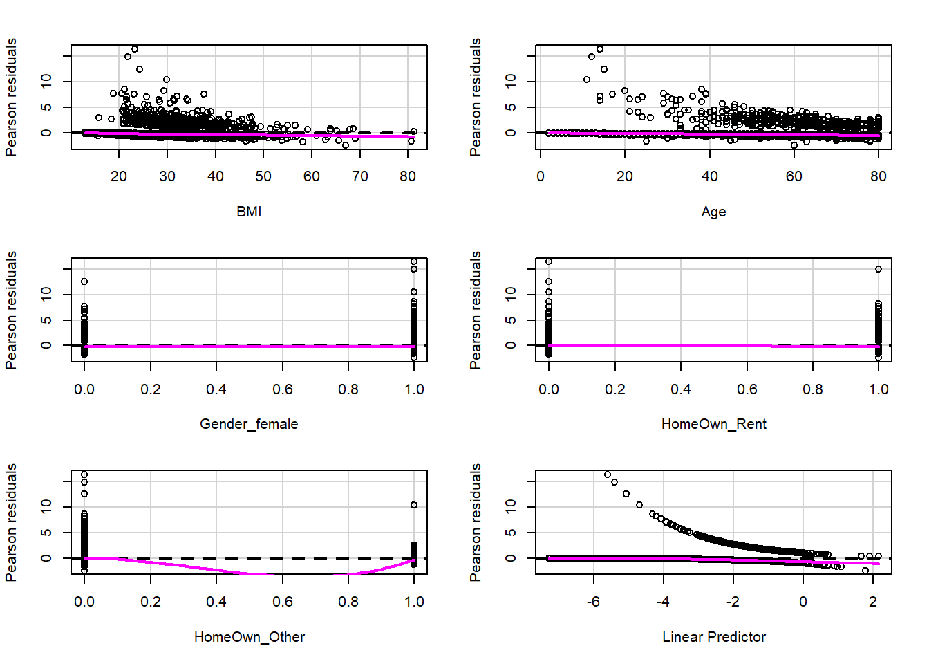
##               Test stat Pr(>|Test stat|)
## BMI              2.5844           0.1079
## Age             20.0291        7.627e-06 ***
## Gender_female    0.0000           1.0000
## HomeOwn_Rent     0.0000           1.0000
## HomeOwn_Other    0.0000           1.0000
## ---
## Signif. codes:  0 '***' 0.001 '**' 0.01 '*' 0.05 '.' 0.1 ' ' 1
The residual plots that you see above can help us visually identify if there are any noticeable relationships between our residuals and independent variables. Any noticeable relationships would indicate a possible lack of fit. We also receive a table as part of the output which shows us the results of a lack of fit test that is conducted for each independent variable.171
We can write the hypotheses for the lack of fit test like this:
- \(H_0\): The independent variable fits the data well.
- \(H_A\): The independent variable does not fit the data well.
The p-value of the lack of fit test for the BMI variable is 0.11, which perhaps hints at support for lack of fit, but overall is not enough support to reject the null hypothesis. The p-value for the Age variable is extremely low and provides strong support in favor of the alternate hypothesis that Age does not fit well in this model. A logical next step could be to add a squared term for Age and re-run the logistic regression model to see if this improves the fit. We will ignore the results of the lack of fit test for any dummy variables.
11.6.3 Marginal model plots
Next, we create marginal model plots for our logistic regression model:
marginalModelPlots(logit)## Error in smooth.construct.tp.smooth.spec(object, dk$data, dk$knots) :
## A term has fewer unique covariate combinations than specified maximum degrees of freedom
## Error in smooth.construct.tp.smooth.spec(object, dk$data, dk$knots) :
## A term has fewer unique covariate combinations than specified maximum degrees of freedom## Error in smooth.construct.tp.smooth.spec(object, dk$data, dk$knots) :
## A term has fewer unique covariate combinations than specified maximum degrees of freedom
## Error in smooth.construct.tp.smooth.spec(object, dk$data, dk$knots) :
## A term has fewer unique covariate combinations than specified maximum degrees of freedom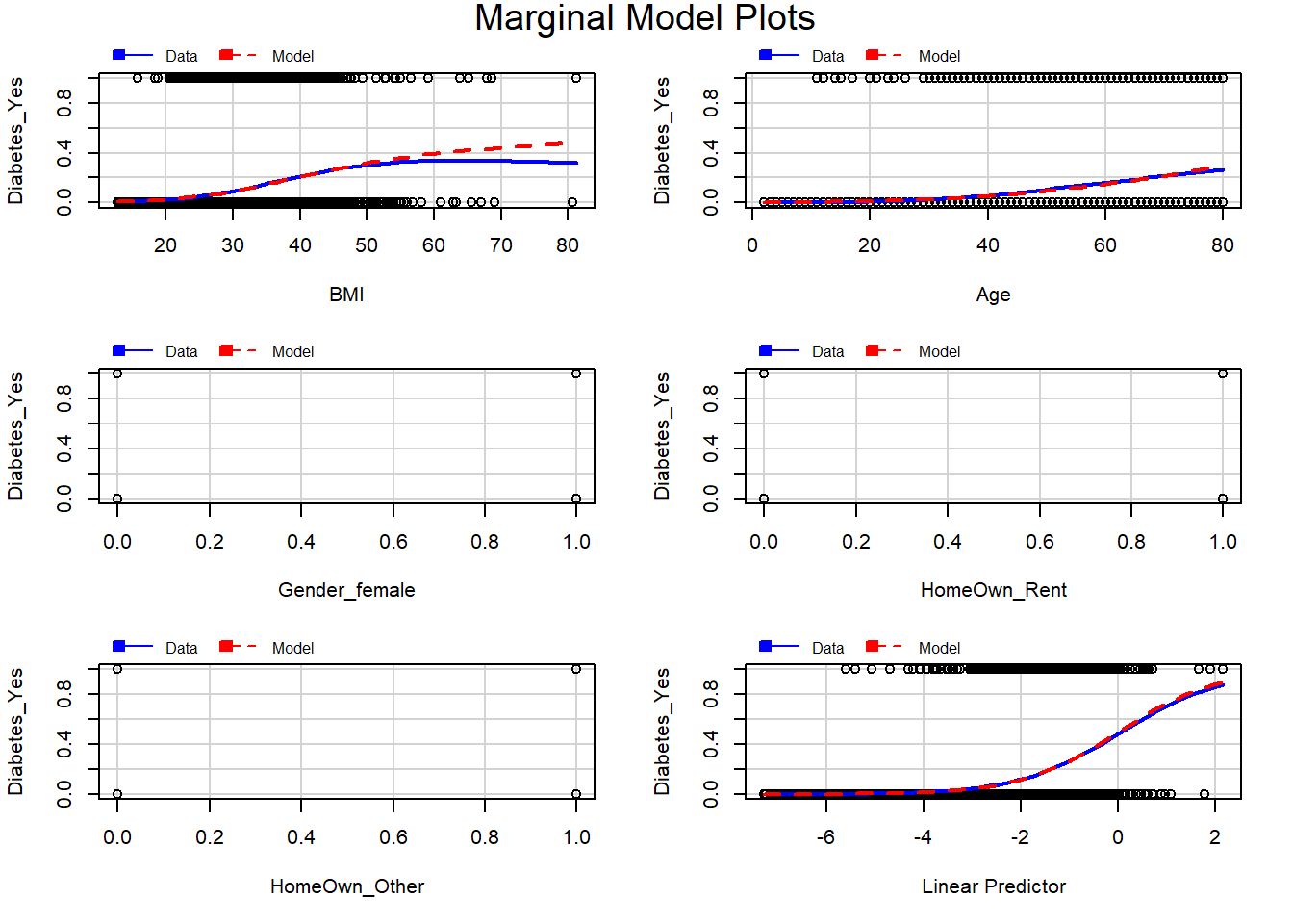
Above, we received plots showing the relationship between our dependent variable and our independent variables, one at a time. In each plot, the computer has created a solid blue line which estimates the relationship between the dependent variable and an independent variable. The dotted red line shows the predictions for this relationship made by our model. We ideally want the blue and red lines to be overlapping with each other.172
Above, we see that for BMI, the blue and red lines deviate at higher levels of BMI. To attempt to fix this problem, we should re-run our regression model and add a squared term for BMI.
11.6.4 Multicollinearity
Since multicollinearity relates only to relationships among the independent variables, we can test it for logistic regression exactly the same way as we previously did for OLS linear regression. This process is presented below in abbreviated form only, since we already learned about this when we learned about OLS diagnostics.
First, we make a correlation matrix with our continuous numeric independent variables:
df1.ind.cont <- df1[c("BMI","Age")]
cor(df1.ind.cont)
## BMI Age
## BMI 1.0000000 0.4106242
## Age 0.4106242 1.0000000Age and BMI are somewhat highly correlated, at 0.41. Let’s see if this is reflected in our VIF metrics:
vif(logit)## BMI Age Gender_female HomeOwn_Rent HomeOwn_Other
## 1.036135 1.144885 1.019331 1.124131 1.016937Above, we see that all of the VIF numbers are quite low, suggesting that multicollinearity is not a problem in our logistic regression model logit. If any of the VIF numbers had been higher than approximately 4, then we would want to consider respecifying our model before we could trust it for inference.
11.6.5 Outliers and influence
There are many possible ways to identify outliers and observations that may be having undesired influence on our regression results. A selection of these methods is demonstrated below. All of these methods use different strategies to identify observations that might be problematic. Every time a test flags an observation as potentially problematic, we should further investigate that observation to see if there is anything wrong with how it is coded or if it does not belong in our sample. We should also re-run our regression model without any influential observations to see if doing so changes our results.
We can generate a series of plots using the influenceIndexPlot(...) function:
influenceIndexPlot(logit)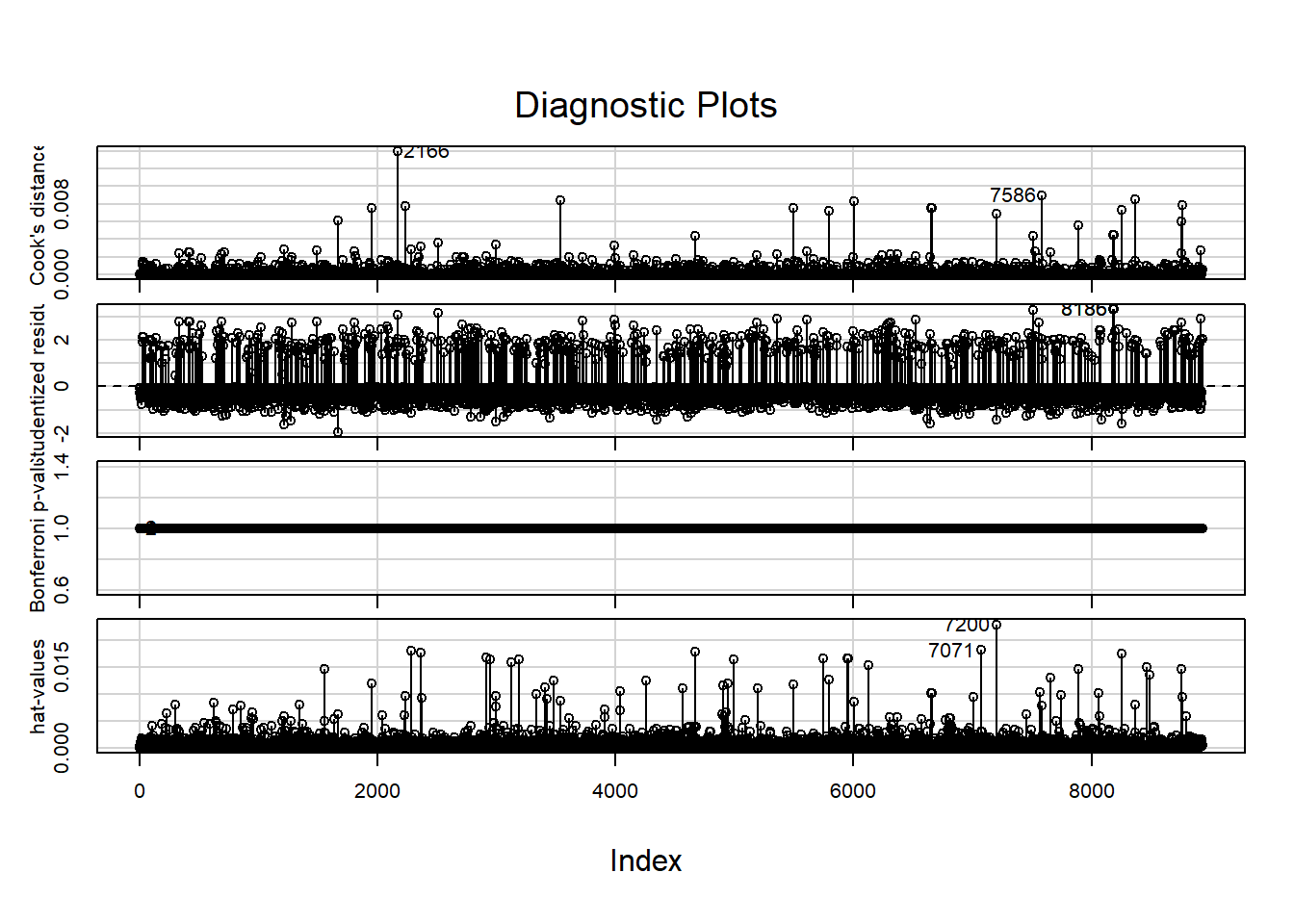
Most of the plots and quantities above can be interpreted as they were for linear regression. Any observations that deviate from the majority of the others in the plots above warrant further attention. The computer also labels the observations that might require more attention.
Another useful test is performed by the outlierTest(...) function:
outlierTest(logit)## No Studentized residuals with Bonferroni p < 0.05
## Largest |rstudent|:
## rstudent unadjusted p-value Bonferroni p
## 8185 3.350996 0.00080521 NAAbove, we receive a list of observations that might warrant further attention.
We can further identify key observations using the influencePlot(...) function:
influencePlot(logit)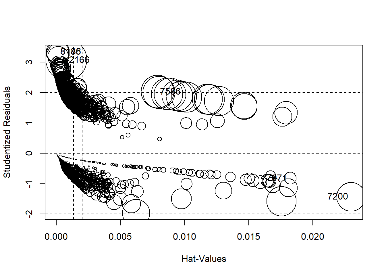
##         StudRes          Hat       CookD
## 2166  3.0794054 0.0007713808 0.014018978
## 7071 -0.8149212 0.0182335977 0.001225823
## 7200 -1.4288008 0.0229827829 0.006900673
## 7586  2.0353683 0.0078699200 0.008963638
## 8185  3.3509962 0.0000985941 0.004433907
## 8186  3.3509962 0.0000985941 0.004433907
Above, we see a plot of studentized residuals against hat values (which tell us the leverage of observations), with the circle size for each observation corresponding to its Cook’s distance.173 We also receive a table that lists observations that may be problematic.
The results of all of the methods above to identify outliers and/or influential observations need to be taken into consideration together. All potentially problematic observations, identfied by any of the tests, need to be examined carefully. A decision then needs to be carefully made about whether or not to include these observations in the logistic regression model.
11.7 Assignment
In this assignment, you will practice creating and interpreting the results of a logistic regression model and assessing goodness of fit. You are permitted to use your own data if you wish and if it is well-suited for binary logistic regression. If you prefer not to use your own data, you will continue to use the NHANES data that was used as an example in this chapter. You will use the variable PhysActive as your dependent variable for this assignment.
11.7.1 Load, prepare, and explore your data
Task 1: Load the NHANES data in R on your computer.
Task 2: Make a copy of the NHANES data called d. You will use the new dataset d for the rest of the assignment.
Task 3: Recode the dependent variable PhysActive into a dummy variable, for you to use in a logistic regression model later in the assignment. Store the new dummy variable in your dataset d.
Task 4: Run the command ?NHANES to read about all of the variables in the dataset. Identify at least two continuous numeric and two categorical variables that you suspect might be associated with our outcome of interest, physical activity. These variables that you choose will be your independent variables in the logistic regression model you make.
Task 5: Write the question of interest that you have decided to answer using a logistic regression model. Keep in mind that PhysActive must be your dependent variable.
Task 6: Remove all unnecessary variables from d. Remember that you can do this by using the code d <- d[c("Var1","Var2","Var3",...)].
Task 7: Use the na.omit(...) function to remove all observations with missing values of your required variables. It is critical to only do this task after you have removed all unnecessary variables.
Task 8: This task is optional (not required). Descriptively explore your data by making at least a total of four visualizations, two-way tables, or other summary statistics. You will run a total of four commands. For example, you might create one visualization and three two-way tables.
11.7.2 Logistic regression model creation and interpretation
Task 9: Run a logistic regression to answer your question of interest. Save this as logit1. Create a summary table of logit1 that shows the estimated coefficients in logit form. Also create a summary table of logit1 that shows odds ratios and 95% confidence intervals for those odds ratios.
Task 10: For your sample, interpret the estimated odds ratios for all independent variables in logit1.
Task 11: For your population of interest, interpret the relationship between the dependent variable and each independent variable in logit1.
Task 12: Interpret the p-value for each independent variable in your logit1 summary table.
11.7.3 Predicted values and goodness of fit
Task 13: Calculate Pseudo-\(R^2\) for logit1 using R. Interpret what Pseudo-\(R^2\) means.
Task 14: Run and interpret the results of the Hosmer-Lemeshow test on logit1.
11.7.4 Follow up and submission
You have now reached the end of this week’s assignment. The tasks below will guide you through submission of the assignment and allow us to gather questions and/or feedback from you.
Task 15: Please write any questions you have for the course instructors (optional).
Task 16: Please write any feedback you have about the instructional materials (optional).
Task 17: Knit (export) your RMarkdown file into a format of your choosing.
Task 18: Please submit your assignment to the D2L assignment drop-box corresponding to this chapter and week of the course. And remember that if you have trouble getting your RMarkdown file to knit, you can submit your RMarkdown file itself. You can also submit an additional file(s) if needed.
There are a number of quantitative methods that can do this, and many are what we would call machine learning techniques, which is the focus of the course HE-930 at MGHIHP.↩︎
Note that if a dependent variable is numeric but fractions are not possible outcomes, linear regression is not always the best model to use.↩︎
StatQuest: Logistic Regression. StatQuest with Josh Starmer. Mar 5, 2018. YouTube. https://www.youtube.com/watch?v=yIYKR4sgzI8.↩︎
StatQuest: Maximum Likelihood, clearly explained!!!. StatQuest with Josh Starmer. Jul 31, 2017. YouTube. https://www.youtube.com/watch?v=XepXtl9YKwc.↩︎
Section 1.3, p. 12 in: Menard, S. (2002). Applied logistic regression analysis (Vol. 106). Sage.↩︎
Section 1.3, pp. 12–13 in: Menard, S. (2002). Applied logistic regression analysis (Vol. 106). Sage.↩︎
Section 1.3, p. 13 in: Menard, S. (2002). Applied logistic regression analysis (Vol. 106). Sage.↩︎
Section 1.3, p. 13 in: Menard, S. (2002). Applied logistic regression analysis (Vol. 106). Sage.↩︎
Body mass index.↩︎
Body mass index.↩︎
Body mass index.↩︎
When this chapter was initially published, “sample” was accidentally written here instead of “population.” The mistake was corrected on February 17 2021.↩︎
There are multiple ways to calculate Pseudo-\(R^2\) and McFadden Pseudo-\(R^2\) is one of them.↩︎
This paragraph as well as the table below it were added in March 2021, later than when this chapter was used in HE902 in spring 2021.↩︎
The p-value is in the column labeled
Pr(>Chisq).↩︎This section was added to this chapter of this textbook on approximately March 5 2021. It was previously a part of Chapter 11. ↩︎
The same is the case for \(\text{R}^2\) for linear models.↩︎
p. 90 in: Menard, S. (2002). Applied logistic regression analysis (Vol. 106). Sage.↩︎
Stoltzfus, J. C. (2011). Logistic regression: a brief primer. Academic Emergency Medicine, 18(10), 1099-1104.↩︎
Stoltzfus, J. C. (2011). Logistic regression: a brief primer. Academic Emergency Medicine, 18(10), 1099-1104.↩︎
Menard, S. (2002). Applied logistic regression analysis (Vol. 106). Sage.↩︎
Menard, S. (2002). Applied logistic regression analysis (Vol. 106). Sage.↩︎
Stoltzfus, J. C. (2011). Logistic regression: a brief primer. Academic Emergency Medicine, 18(10), 1099-1104.↩︎
Menard, S. (2002). Applied logistic regression analysis (Vol. 106). Sage.↩︎
Menard, S. (2002). Applied logistic regression analysis (Vol. 106). Sage.↩︎
Menard, S. (2002). Applied logistic regression analysis (Vol. 106). Sage.↩︎
Menard, S. (2002). Applied logistic regression analysis (Vol. 106). Sage.↩︎
Menard, S. (2002). Applied logistic regression analysis (Vol. 106). Sage.↩︎
Stoltzfus, J. C. (2011). Logistic regression: a brief primer. Academic Emergency Medicine, 18(10), 1099-1104.↩︎
Section 8.6.1 “Residuals and Residual Plots,” p. 574/802, in: Fox, J. and Weisberg, S. (2019) An R Companion to Applied Regression, Third Edition, Sage.↩︎
Section 8.2.2 “Marginal-Model Plots,” p. 537/802, in: Fox, J. and Weisberg, S. (2019) An R Companion to Applied Regression, Third Edition, Sage.↩︎
Zhang, Z. (2016). Residuals and regression diagnostics: focusing on logistic regression. Annals of translational medicine, 4(10).↩︎