Chapter 7 Mar 1–7: Correlation and Simple OLS Linear Regression

This chapter is now ready for use by students in HE-802 in spring 2021.

This week, our goals are to…

Examine the process that OLS linear regression uses to draw a line of best fit.
Run a simple OLS linear regression in R and interpret its coefficient estimates.
Interpret goodness-of-fit metrics for OLS linear regression.

Announcements and reminders

This chapter contains more information than you need to know about OLS regression. I suggest that you look through the tasks in the assignment first and then use that to help you determine what to read in the chapter.
We will have group Zoom sessions this week at 5:00 p.m. Boston time on Wednesday and Friday. You should have received calendar invitations from Nicole for these sessions. Remember that you can always contact us to schedule additional group or one-on-one sessions at other times.

7.1 Ordinary least squares (OLS) line of best fit

One of the most important concepts that we will be learning and applying throughout this textbook is regression analysis. More specifically, linear regression is the most common form are for regression analysis that we will use. The purpose of linear regression is to fit a linear equation to a set of data.

You may recall that the most basic form of a linear equation can be written as $y=mx+b$ or $y=b_1x+b_0$. $m$ or $b_1$ refers to the slope of the line. $b$ or $b_0$ refers to the y-intercept of the line (the y-intercept can also be called just the intercept or the constant). For every one unit increase in X, Y increases by $m$ (or $b_1$) units. Remember that these words—“For every one unit increase in X”—are the magic words.

The most common type of linear regression is called OLS linear regression. OLS stands for ordinary least squares. This type of linear regression attempts to fit a line to our data that is as close to as many of the data points as possible. It uses the least squares method to fit the line. You will gain an intuition for the least squares method as you encounter the examples that follow in this chapter.

Below are a few videos that are optional (not required) for you to watch, if you feel that a few audio-visual examples might be useful. We will also walk through the steps and interpretation of linear regression later in the chapter. Some of these videos will give you a sense for how linear regression models are calculated and interpreted. Note that all of these videos were created by different instructors, for different audiences.

This video carefully walks through how a regression line is calculated:⁸⁹

The video above can be viewed externally at https://youtu.be/JvS2triCgOY.

And this video also demonstrates the calculation of the least squares regression line in a different way:⁹⁰

The video above can be viewed externally at https://www.youtube.com/watch?v=jEEJNz0RK4Q.

This video explains how we can analyze the extent to which there is error in a regression line, in addition to discussing regression more generally:⁹¹

The video above can be viewed externally at https://www.youtube.com/watch?v=coQAAN4eY5s.

You will frequently have to interpret regression results that were produced by computer programs. The following video focuses on how to interpret these results:⁹²

The video above can be viewed externally at https://youtu.be/sIJj7Q77SVI.

7.2 Simple OLS linear regression in R

In this section, we will run a simple OLS linear regression model in R and interpret the results. We will continue with the data and example that we used earlier in this chapter. Note that “simple” OLS regression refers to a regression analysis in which there is only one independent variable, which is the focus of this section. It is fine to refer to a regression model with one independent variable as a simple OLS linear regression, simple linear regression, OLS linear regression, or linear regression. All of these terms mean the same thing. The terms regression analysis and regression model can also be used interchangeably. They mean the same thing, for our purposes.

Here are the key details of the example regression analysis we will conduct:

Question: What is the association between displacement and weight in cars?
Dependent variable: disp; displacement in cubic inches.
Independent variable: wt; weight in tons.
Dataset: mtcars data in R, loaded as d in our example. Run the code d<-mtcars if you have not already, to load the data.

Let’s create a dataset called d which is a copy of mtcars:

d <- mtcars

We can inspect our entire dataset d with the following command:

View(d)

7.2.1 OLS in our sample

Let’s start by making a linear regression model on our sample with the R code below:

reg1 <- lm(disp~wt, data = d)

Here is what we are telling the computer to do with the code above:

reg1 – Create a new regression object called reg1. This can be named anything, not necessarily reg1.
<- – Assign reg1 to be the result of the output of the function lm(...)
lm(...) – Run a linear model using OLS linear regression.
disp – This is the dependent variable in the regression model.
~ – This is part of a formula. This is like the equals sign within an equation.
wt – This is the independent variable in the regression model.
data = d – Use the dataset d for this regression. d is where the dependent and independent variables are located.

If you look in the Environment tab in RStudio, you will see that reg1 is saved and listed there. Our regression results are stored as the object reg1 in R and we can refer back to them any time we want, as we will be doing multiple times below.

We are now ready to inspect the results of our regression model by using the summary(...) function to give us a summary of reg1, like this:

summary(reg1)

## 
## Call:
## lm(formula = disp ~ wt, data = d)
## 
## Residuals:
##    Min     1Q Median     3Q    Max 
## -88.18 -33.62 -10.05  35.15 125.59 
## 
## Coefficients:
##             Estimate Std. Error t value Pr(>|t|)    
## (Intercept)  -131.15      35.72  -3.672 0.000933 ***
## wt            112.48      10.64  10.576 1.22e-11 ***
## ---
## Signif. codes:  0 '***' 0.001 '**' 0.01 '*' 0.05 '.' 0.1 ' ' 1
## 
## Residual standard error: 57.94 on 30 degrees of freedom
## Multiple R-squared:  0.7885, Adjusted R-squared:  0.7815 
## F-statistic: 111.8 on 1 and 30 DF,  p-value: 1.222e-11

Above, we see summary output of our regression model. The most important section that we will look at first is the Coefficients section of the output. In the linear equation $y=mx+b$, $m$ and $b$ are called coefficients. In the linear equation $y=b_1x+b_0$, $b_1$ and $b_0$ are called coefficients. For the rest of our work together, we will use the $y=b_1x+b_0$ version of the linear equation.

We learn the following details from the Coefficients section of the regression output:

$b_0 = -131.15$ – This means that the intercept⁹³ is -131.15.
$b_1 = 112.48$ – This means that the slope of wt is 112.48.

We can follow these steps to write this regression result as an equation:

Start with the generic form of the linear equation: $y=b_1x+b_0$
Replace $b_0$ and $b_1$ with the corresponding numbers from the regression output: $y=112.48x-131.15$
Replace $y$ and $x$ with the correct variable names from our dataset: $disp=112.48wt-131.15$
Add a hat to the dependent variable, to indicate that this equation calculates predicted values (rather than actual values) of the dependent variable: $\hat{disp}=112.48wt-131.15$

$\hat{disp}=112.48wt-131.15$ is the final equation. This equation defines the line that bests fits our data in our sample, according to the OLS linear regression method.

Now we can interpret these results by looking at the equation:

Slope of wt: For every one ton increase in weight, displacement is predicted to increase by 112.48 cubic inches in our sample.
Intercept: When weight is equal to 0 tons, the predicted value of displacement is -131.15 cubic inches in our sample. This prediction of a negative number doesn’t make sense, of course. We are typically more interested in knowing the slope rather than the intercept of a regression model, because the slope is typically going to be what helps us answer our question of interest.⁹⁴

You should always start with the magic words “For every one unit increase in X…” when you are interpreting regression results.

Note that we did NOT prove that the independent variable weight is causing the dependent variable displacement. We only found that there is an association between these two variables in our sample.⁹⁵

We can do a little bit of basic math on our regression equation to see that the slope and intercept above are correct. We do this by plugging hypothetical numbers into the regression equation. Let’s imagine a car that weighs 2 tons and that we want to use our regression equation to calculate the predicted displacement for this car. We do this by substituting the number 2 in place of $wt$ in our equation:

$\hat{disp}=112.48*2-131.15 = 93.81$

This means that our regression model predicts that when a car weighs 2 tons, it has a displacement of 93.81 cubic inches.

Below, we plug in a few different values for $wt$ in our equation $\hat{disp}=112.48wt-131.15$:

$wt$	Calculation	$\hat{disp}$	Interpretation
0	$\hat{disp}=112.48*0-131.15 = -131.15$	-131.15 cubic inches	When a car weighs 0 tons, it has a predicted displacement of -131.15 cubic inches. This is the intercept of our regression result. In this case, the intercept is not particularly meaningful, because there is no such thing as a car that weighs 0 tons.
1	$\hat{disp}=112.48*1-131.15 = -18.67$	-18.67 cubic inches	When a car weighs 1 ton, it has a predicted displacement of -18.67 cubic inches.
2	$\hat{disp}=112.48*2-131.15 = 93.81$	93.81 cubic inches	When a car weighs 2 tons, it has a predicted displacement of 93.81 cubic inches.
3	$\hat{disp}=112.48*3-131.15 = 206.29$	206.29 cubic inches	When a car weighs 3 tons, it has a predicted displacement of 206.29 cubic inches.

We can make the following observations about the table above:

When we change the weight from 0 to 1, the predicted displacement changes from -131.15 to -18.67. This change is a difference of $-18.67-(-131.15) = 112.48$.
When we change the weight from 1 to 2, the predicted displacement changes from -18.67 to 93.81. This change is a difference of $93.81-(-18.67) = 112.48$.
When we change the weight from 2 to 3, the predicted displacement changes from 93.81 to 206.29. This change is a difference of $206.29-93.81 = 112.48$.
We could keep going like this and we would always find that when we increase weight by one ton, predicted displacement would increase by 112.48.

The calculations above confirm that 112.48 cubic inches is the slope of the association between displacement and weight in our sample.

Our equation $\hat{disp}=112.48wt-131.15$ tells us the exact relationship on average between displacement and weight in our sample. Everything written above has pertained to our sample only. We will now turn our attention to inference and our population of interest.

7.2.2 OLS in our population

We are now interested in answering this question: What is the true relationship between displacement and weight in the population from which our sample was selected?

To answer this question, we have to look at some of the inferential statistics that are calculated when we do a regression analysis. We also need to conduct some diagnostic tests of assumptions before we can trust the results.

We will start by calculating the 95% confidence intervals for our estimated regression coefficients, by running the confint(...) function on our saved regression results—called reg1—like this:

confint(reg1)

##                 2.5 %   97.5 %
## (Intercept) -204.0914 -58.2054
## wt            90.7579 134.1984

It is also possible to create a regression summary table that contains everything we need all in one place, using the summ(...) function from the jtools package.

Run the following code to load the package and see our regression results:

if (!require(jtools)) install.packages('jtools')
library(jtools)

summ(reg1, confint = TRUE)

Observations	32
Dependent variable	disp
Type	OLS linear regression

F(1,30)	111.85
R²	0.79
Adj. R²	0.78

	Est.	2.5%	97.5%	t val.	p
(Intercept)	-131.15	-204.09	-58.21	-3.67	0.00
wt	112.48	90.76	134.20	10.58	0.00
Standard errors: OLS

Here is what the lines of code above accomplished:

if (!require(jtools)) install.packages('jtools') – Check if the jtools package is already installed and install it if not.
library(jtools) – Load the jtools package.
summ(reg1, confint = TRUE) – Create a summary output of the saved reg1 regression result. Include the confidence intervals (because confint is set to TRUE).

We can now interpret the 95% confidence intervals that were calculated:

Slope: In the population from which our sample was drawn, we are 95% confident that the slope of the relationship between displacement and weight is between 90.76 and 134.20 cubic inches. In other words: In our population of interest, we are 95% confident that for every one ton increase in a car’s weight, its displacement is predicted to increase by at least 90.76 cubic inches or at most 134.20 cubic inches. This is the answer to our question of interest, if our data passes all diagnostic tests that we will conduct later.
Intercept: In the population from which our sample was drawn, we are 95% confident that the intercept of the relationship between displacement and weight is between -204.09 and -58.21 cubic inches. In other words: In our population of interest, we are 95% confident that a car that weighs 0 tons has a displacement between -204.09 and -58.21 cubic inches. Of course, this intercept is not very meaningful to us (which is fine) because there is no such thing as a car that is weightless.⁹⁶

Note that we did NOT prove that the independent variable weight is causing the dependent variable displacement. We only found that there is potentially—not definitely—an association between these two variables in our population of interest.⁹⁷

The computer conducted a number of hypothesis tests for us when it ran our regression analysis. The most important of these hypothesis tests relates to the slope estimate for displacement and weight.

Here is the framework for this hypothesis test:

$H_0$: In the population of interest, $b_1 = 0$. In other words: in the population of interest, there is no relationship between displacement and weight of cars.
$H_A$: In the population of interest, $b_1 \ne 0$. In other words: in the population of interest, there is a non-zero relationship between displacement and weight of cars.

We find the result of this hypothesis test within the regression output. The p-value for weight is extremely small, listed as 0.00 in one summary table and 1.22e-11 in another. This means that we have very high confidence in the alternate hypothesis $H_A$, meaning that there likely is an association between displacement and weight in our population of interest. More specifically, we are 95% confident that the slope of the association between displacement and weight in the population is between 90.76 and 134.20 cubic inches. Taking the p-value and confidence intervals into consideration, we reject the null hypothesis.

Here are some important reminders about our OLS linear regression results:

All of the estimated coefficients are measured in units of the dependent variable.
The slope of 112.48 cubic inches is the true average relationship between displacement and weight in our sample alone.
The 95% confidence intervals and p-values pertain to the population.
The slope of 112.48 cubic inches is the midpoint of the 95% confidence interval.⁹⁸
None of these results for the population of interest can be trusted until certain diagnostic tests of assumptions have been conducted.

7.2.3 Graphing OLS results

We can also graph the results of our OLS regression on a scatterplot. And this scatterplot will help us visualize some key characteristics about our regression line.

To make the plot of our data points and regression line, run this code:

plot(d$wt,d$disp)
abline(reg1)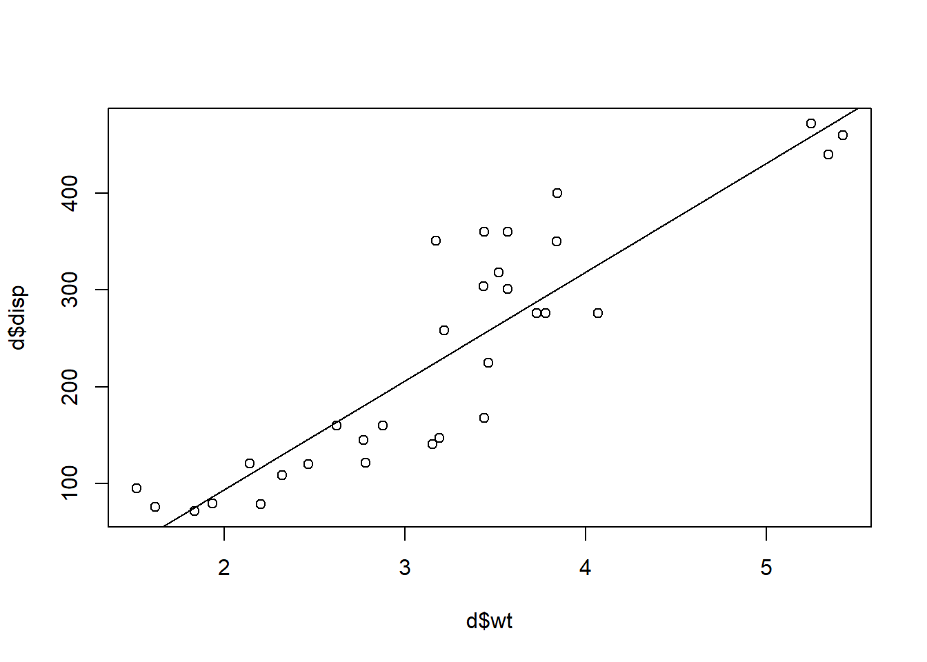

Here is what the code above asked the computer to do:

plot(d$wt,d$disp) – Create a scatterplot with d$wt on the horizontal axis and d$disp on the vertical axis.
abline(reg1, col = 'blue') – Add the regression line for reg1 to the already created scatterplot.

The scatterplot shows that the regression line fits the data pretty well. Most of the points are pretty close to the line. This means that there is not much error in the regression line. Such a well-fitting result is not common in social science, behavioral science, health, and education data.

7.2.4 Generic code for OLS linear regression in R

This section contains a generic version of the code and interpretation that you can use to run a simple OLS linear regression in R. You can copy the code below and follow the guidelines to replace elements of this code such that it is useful for analyzing your own data.

To run an OLS linear regression in R, you will use the lm(...) command:

reg1 <- lm(DepVar ~ IndVar, data = mydata)

Here is what we are telling the computer to do with the code above:

reg1 – Create a new regression object called reg1. You can call this whatever you want. It doesn’t need to be called reg1.
<- – Assign reg1 to be the result of the output of the function lm(...)
lm(...) – Run a linear model using OLS linear regression.
DepVar – This is the dependent variable in the regression model. You will write the name of your own dependent variable instead of DepVar.
~ – This is part of a formula. This is like the equals sign within an equation.
IndVar – This is the independent variable in the regression model. You will write the name of your own independent variable instead of IndVar.
data = mydata – Use the dataset mydata for this regression. mydata is where the dependent and independent variables are located. You will replace mydata with the name of your own dataset.

Then we would run the following command to see the results of our saved regression, reg1:

summary(reg1)

The summary(...) function shows you the results of the regression that you created and saved as reg1.

If you look in your Environment tab in RStudio, you will see that reg1 (or whatever you called your regression) is saved and listed there.

A summary table with confidence intervals can be created with the following code:

if (!require(jtools)) install.packages('jtools')
library(jtools)

summ(reg1, confint = TRUE)

7.3 OLS residuals

We will continue using the reg1 regression model that we created earlier in this chapter, which examined the relationship between displacement and weight of cars. Earlier in the chapter, our focus was on interpreting the slope and intercept in the regression model. Now we will turn our attention to an analysis of the individual observations in our dataset. Below, we will examine errors between our actual and predicted values of displacement in our regression model.

Remember: Displacement (disp) is our dependent variable and weight (wt) is our independent variable in this regression model. The dependent variable is our outcome of interest that we care about. Our main concern when we analyze residuals and error is our predictions of the dependent variable made by the regression model. Most of the procedure below is based on the dependent variable alone, which is displacement (disp).⁹⁹

Earlier in the chapter, we calculated predicted values of hypothetical cars that weighed 0, 1, 2, and 3 tons. We did this by plugging these numbers in for $weight$ into our regression equation $\hat{disp}=112.48wt-131.15$. Now we are going to plug the actual (real, not predicted) values of weight for the observations in our dataset and plug those into our regression equation. This process generates what is called the predicted values or fitted values of our regression model.¹⁰⁰

Here we calculate predicted values in R:

d$disp.predicted <- predict(reg1)

Here’s what the code above did:

d$disp.predicted <- – Create a new variable called disp.predicted within the dataset d. The new variable will be assigned the values of the code to the right of the <- operator.
predict(reg1) – Calculate predicted values for the regression model reg1.

Now a new variable called disp.predicted has been added to our dataset d. You can inspect this new variable by opening d in R on your own computer, using the View(...) command:

View(d)

In the table below, you can see our independent variable (wt), dependent variable (disp), and predicted values of the dependent variable (disp.predicted).

d[c("wt","disp","disp.predicted")]

                   wt  disp disp.predicted

Mazda RX4 2.620 160.0 163.54431 Mazda RX4 Wag 2.875 160.0 192.22623 Datsun 710 2.320 108.0 129.80087 Hornet 4 Drive 3.215 258.0 230.46880 Hornet Sportabout 3.440 360.0 255.77638 Valiant 3.460 225.0 258.02594 Duster 360 3.570 360.0 270.39854 Merc 240D 3.190 146.7 227.65685 Merc 230 3.150 140.8 223.15772 Merc 280 3.440 167.6 255.77638 Merc 280C 3.440 167.6 255.77638 Merc 450SE 4.070 275.8 326.63761 Merc 450SL 3.730 275.8 288.39504 Merc 450SLC 3.780 275.8 294.01895 Cadillac Fleetwood 5.250 472.0 459.36181 Lincoln Continental 5.424 460.0 478.93301 Chrysler Imperial 5.345 440.0 470.04723 Fiat 128 2.200 78.7 116.30349 Honda Civic 1.615 75.7 50.50378 Toyota Corolla 1.835 71.1 75.24897 Toyota Corona 2.465 120.1 146.11020 Dodge Challenger 3.520 318.0 264.77463 AMC Javelin 3.435 304.0 255.21399 Camaro Z28 3.840 350.0 300.76764 Pontiac Firebird 3.845 400.0 301.33003 Fiat X1-9 1.935 79.0 86.49678 Porsche 914-2 2.140 120.3 109.55480 Lotus Europa 1.513 95.1 39.03101 Ford Pantera L 3.170 351.0 225.40728 Ferrari Dino 2.770 145.0 180.41603 Maserati Bora 3.570 301.0 270.39854 Volvo 142E 2.780 121.0 181.54081

In the table above, the final observation is a car called the Volvo 142E. Let’s use this car as an example to see how the computer calculated the predicted value for the Volvo 142E.

Procedure for calculating predicted displacement (dependent variable) for Volvo 142E:

Start with regression equation: $\hat{disp}=112.48wt-131.15$
See that the Volvo 142E weighs 2.780 tons.
Plug 2.780 tons into the regression equation: $\hat{disp}=112.48*2.780-131.15 = 181.54 cubic inches$
The predicted displacement from our regression model of the Volvo 142E is 181.54 cubic inches.

Here is what we know about the Volvo 142E:

Weight: $wt = 2.780\text{ tons}$. This is how much the Volvo 142E truly weighs in reality.
Actual displacement: $disp = 121.0\text{ cubic inches}$. This is how much displacement the Volvo 142E truly has in reality.
Predicted displacement: $\hat{disp} = 181.54\text{ cubic inches}$. This is how much displacement the regression model “thinks” the Volvo 142E has.

Remember that you saw the scatterplot of the data points and the regression line. In that scatterplot, there was some distance between the points and the line in most cases. We are now about to calculate the distances between the points and the line.

For the Volvo 142E, the actual value (the plotted point) of disp—called $disp$—is 121.0 cubic inches; and the predicted value from the regression equation of disp—called $\hat{disp}$—is 181.54 cubic inches. This means that there is some error.

Here are a few ways to write the error:

$Error = Actual - Predicted = 121.0 - 181.54 = -60.54$
$\epsilon = disp - \hat{disp} = 121.0 - 181.54 = -60.54$

Above, $\epsilon$ means error. $disp$ means actual value of displacement. $\hat{disp}$ means predicted value of displacement. The hat over a variable’s name means that it is a predicted value. Notice that this analysis of error so far has related to the dependent variable (our outcome of interest). We calculate errors for the dependent variable only.¹⁰¹

The error for the Volvo 142E is -60.54. This is called the residual for the Volvo 142E. Our goal in OLS linear regression is to make a line for which the residual values for all of the observations are—overall—as low as possible. Now we will calculate and analyze the residuals for all of the observations in the data. The terms, residual values, residuals, and residual errors can all be used to mean the same thing, in the context of regression.

We run the following code to calculate the regression residuals:

d$disp.resid <- resid(reg1)

Here’s what we asked the computer to do with the code above:

d$disp.resid <- – Create a new variable called disp.resid within the dataset d. The new variable will be assigned the values of the code to the right of the <- operator.
resid(reg1) – Calculate residual values for the regression model reg1.

Now a new variable called disp.resid has been added to our dataset d. You can inspect this new variable by opening d in R on your own computer, using the View(...) command:

View(d)

In the table below, you can see our independent variable (wt), dependent variable (disp), predicted values of the dependent variable (disp.predicted), and the residuals (disp.resid):

d[c("wt","disp","disp.predicted","disp.resid")]

                   wt  disp disp.predicted disp.resid

Mazda RX4 2.620 160.0 163.54431 -3.544307 Mazda RX4 Wag 2.875 160.0 192.22623 -32.226232 Datsun 710 2.320 108.0 129.80087 -21.800865 Hornet 4 Drive 3.215 258.0 230.46880 27.531201 Hornet Sportabout 3.440 360.0 255.77638 104.223620 Valiant 3.460 225.0 258.02594 -33.025943 Duster 360 3.570 360.0 270.39854 89.601462 Merc 240D 3.190 146.7 227.65685 -80.956846 Merc 230 3.150 140.8 223.15772 -82.357720 Merc 280 3.440 167.6 255.77638 -88.176380 Merc 280C 3.440 167.6 255.77638 -88.176380 Merc 450SE 4.070 275.8 326.63761 -50.837608 Merc 450SL 3.730 275.8 288.39504 -12.595040 Merc 450SLC 3.780 275.8 294.01895 -18.218947 Cadillac Fleetwood 5.250 472.0 459.36181 12.638189 Lincoln Continental 5.424 460.0 478.93301 -18.933007 Chrysler Imperial 5.345 440.0 470.04723 -30.047234 Fiat 128 2.200 78.7 116.30349 -37.603489 Honda Civic 1.615 75.7 50.50378 25.196222 Toyota Corolla 1.835 71.1 75.24897 -4.148968 Toyota Corona 2.465 120.1 146.11020 -26.010195 Dodge Challenger 3.520 318.0 264.77463 53.225369 AMC Javelin 3.435 304.0 255.21399 48.786010 Camaro Z28 3.840 350.0 300.76764 49.232364 Pontiac Firebird 3.845 400.0 301.33003 98.669974 Fiat X1-9 1.935 79.0 86.49678 -7.496782 Porsche 914-2 2.140 120.3 109.55480 10.745200 Lotus Europa 1.513 95.1 39.03101 56.068992 Ford Pantera L 3.170 351.0 225.40728 125.592717 Ferrari Dino 2.770 145.0 180.41603 -35.416028 Maserati Bora 3.570 301.0 270.39854 30.601462 Volvo 142E 2.780 121.0 181.54081 -60.540809

In the final row of the table above, you can see that the computer calculated the same residual value for the Volvo 142E that we had calculated ourselves, -60.54 cubic inches. The computer has also calculated for us the residual value of all observations. You can choose a few other observations and calculate for yourself. You will find that the residual is always the difference between the actual and predicted value for each observation.

The residuals in a regression analysis will be useful to us as we run a variety of analyses.

7.4 R-squared metric of goodness of fit in OLS

All regression models have a variety of goodness-of-fit measures that help us understand how well a regression model fits our data and/or how appropriate it is for our data. In this section, we will learn about the measure called $R^2$. This measure is referred to as “R-squared,” “R-square,” “Multiple R-squared,” or something similar. They all mean the same thing.

If you look at the summary table that we made for reg1, you will see that it says Multiple R-squared: 0.7885. This number can also be interpreted as 78.9%. This means that 78.9% of the variation in the Y variable (disp) is accounted for by variation in the X variable (wt). This is a very high $R^2$ in the context of social science, behavioral, health, and education data. Every time you run an OLS regression (and many other types of regressions as well), you should examine the $R^2$ statistic to see how well your regression model fits your data.

The $R^2$ statistic tells us how well our independent variable helps us predict the value of our dependent variable. Our ultimate goal is to make good predictions of the dependent variable by fitting the best regression line possible to the data. Once you know the $R^2$ of a regression model, you can also use that to compare it to other regression models to see which model has the better fitting line. We will practice doing this later in this textbook.¹⁰²

$R^2$ has an interesting connection to correlation. $R^2$ is the square of the correlation of the actual and predicted values in any OLS linear regression. We will demonstrate this by calculating in R, below.

7.4.1 Correlation and R-squared

We have already calculated the predicted values from our regression model and added them to our dataset d. Below, we calculate the correlation coefficient of the actual and predicted values of disp in our dataset d.

Here we use the cor(...) function to correlate disp and disp.predicted:

cor(d$disp,d$disp.predicted)

## [1] 0.8879799

And we can also save this correlation as r.reg using this code:

r.reg <- cor(d$disp,d$disp.predicted)

Now r.reg is saved in R’s memory for us to use later if we want. You will see it listed in the environment.

Now we will calculate the square of r.reg:

r.reg^2

## [1] 0.7885083

Above, we see that this square of the correlation of actual and predicted values is the same as the $R^2$ metric from the OLS regression that we ran. Soon—not in this chapter, though—we will be adding more than one independent variable into our regression models. Even with more than one independent variable, the square of the correlation of the actual and predicted values will be equal to the $R^2$ statistic in an OLS linear regression.

7.4.2 Calculating R-squared

Now we will learn how exactly $R^2$ is calculated. To calculate $R^2$, we have to first calculate two values called SSR and SST:

SSR means sum of squares regression.
SST means sum of squares total.

First we will calculate SSR. We begin this process by calculating the squares of all residuals. We had already calculated residuals before, so we just need to create a new variable in our dataset d which is the square of the residuals.

Here is the code to square the residuals:

d$disp.resid2 <- d$disp.resid^2

Here is what the code above is doing:

d$disp.resid2 <- – Create a new variable called disp.resid2 within the dataset d. disp.resid2 will be equal to the value calculated by the code to the right of the <- operator.
d$disp.resid^2 – Square the value of disp.resid for each observation within the dataset d.

We can examine our dataset d with the added new variable disp.resid2—which stands for “displacement residual squared”—by running the View(...) function:

View(d)

Below is a table of d with the new disp.resid2 variable added:

d[c("wt","disp","disp.predicted","disp.resid","disp.resid2")]

                   wt  disp disp.predicted disp.resid disp.resid2

Mazda RX4 2.620 160.0 163.54431 -3.544307 12.56211 Mazda RX4 Wag 2.875 160.0 192.22623 -32.226232 1038.53004 Datsun 710 2.320 108.0 129.80087 -21.800865 475.27773 Hornet 4 Drive 3.215 258.0 230.46880 27.531201 757.96702 Hornet Sportabout 3.440 360.0 255.77638 104.223620 10862.56290 Valiant 3.460 225.0 258.02594 -33.025943 1090.71292 Duster 360 3.570 360.0 270.39854 89.601462 8028.42194 Merc 240D 3.190 146.7 227.65685 -80.956846 6554.01087 Merc 230 3.150 140.8 223.15772 -82.357720 6782.79408 Merc 280 3.440 167.6 255.77638 -88.176380 7775.07405 Merc 280C 3.440 167.6 255.77638 -88.176380 7775.07405 Merc 450SE 4.070 275.8 326.63761 -50.837608 2584.46234 Merc 450SL 3.730 275.8 288.39504 -12.595040 158.63504 Merc 450SLC 3.780 275.8 294.01895 -18.218947 331.93004 Cadillac Fleetwood 5.250 472.0 459.36181 12.638189 159.72383 Lincoln Continental 5.424 460.0 478.93301 -18.933007 358.45875 Chrysler Imperial 5.345 440.0 470.04723 -30.047234 902.83627 Fiat 128 2.200 78.7 116.30349 -37.603489 1414.02236 Honda Civic 1.615 75.7 50.50378 25.196222 634.84962 Toyota Corolla 1.835 71.1 75.24897 -4.148968 17.21394 Toyota Corona 2.465 120.1 146.11020 -26.010195 676.53026 Dodge Challenger 3.520 318.0 264.77463 53.225369 2832.93986 AMC Javelin 3.435 304.0 255.21399 48.786010 2380.07481 Camaro Z28 3.840 350.0 300.76764 49.232364 2423.82570 Pontiac Firebird 3.845 400.0 301.33003 98.669974 9735.76369 Fiat X1-9 1.935 79.0 86.49678 -7.496782 56.20174 Porsche 914-2 2.140 120.3 109.55480 10.745200 115.45931 Lotus Europa 1.513 95.1 39.03101 56.068992 3143.73190 Ford Pantera L 3.170 351.0 225.40728 125.592717 15773.53057 Ferrari Dino 2.770 145.0 180.41603 -35.416028 1254.29501 Maserati Bora 3.570 301.0 270.39854 30.601462 936.44946 Volvo 142E 2.780 121.0 181.54081 -60.540809 3665.18955

Above, we see that for each observation, the value of disp.resid2 is the square of the value of disp.resid.

The next step as we continue to calculate SSR is to calculate the sum of the squared residuals column.

The code below sums up the disp.resid2 column:

sum(d$disp.resid2)

## [1] 100709.1

The sum above is the SSR. The SSR is the sum of all squared residuals. In this data, SSR = 100709.1

Now we will turn to calculating SST. The first step is to determine the mean of the dependent variable, disp.

We can use the mean(...) function to calculate this:

mean(d$disp)

## [1] 230.7219

The next step is to subtract the dependent variable’s value from the mean of the dependent variable for each observation.

This code subtracts the mean from each disp:

d$disp.meandiff <- d$disp-230.7219

Here is what we are asking the computer to do above:

d$disp.meandiff <- – Create a new variable called meandiff in the dataset d which will be equal to the calculated values by the code on the right side of the <- operator.
d$disp-230.7219 – For each observation in d, subtract 230.7219 (which is the mean of the variable disp) from that observation’s value of disp.

The next step is to square the meandiff variable:

d$disp.meandiff2 <- d$disp.meandiff^2

And now we can have a look at our data again. In R, run the View(…) command to inspect our dataset d with all of the new variables included:

View(d)

In the table below we see some of the recently added variables:

d[c("wt","disp","disp.resid","disp.resid2","disp.meandiff","disp.meandiff2")]

                   wt  disp disp.resid disp.resid2 disp.meandiff

Mazda RX4 2.620 160.0 -3.544307 12.56211 -70.7219 Mazda RX4 Wag 2.875 160.0 -32.226232 1038.53004 -70.7219 Datsun 710 2.320 108.0 -21.800865 475.27773 -122.7219 Hornet 4 Drive 3.215 258.0 27.531201 757.96702 27.2781 Hornet Sportabout 3.440 360.0 104.223620 10862.56290 129.2781 Valiant 3.460 225.0 -33.025943 1090.71292 -5.7219 Duster 360 3.570 360.0 89.601462 8028.42194 129.2781 Merc 240D 3.190 146.7 -80.956846 6554.01087 -84.0219 Merc 230 3.150 140.8 -82.357720 6782.79408 -89.9219 Merc 280 3.440 167.6 -88.176380 7775.07405 -63.1219 Merc 280C 3.440 167.6 -88.176380 7775.07405 -63.1219 Merc 450SE 4.070 275.8 -50.837608 2584.46234 45.0781 Merc 450SL 3.730 275.8 -12.595040 158.63504 45.0781 Merc 450SLC 3.780 275.8 -18.218947 331.93004 45.0781 Cadillac Fleetwood 5.250 472.0 12.638189 159.72383 241.2781 Lincoln Continental 5.424 460.0 -18.933007 358.45875 229.2781 Chrysler Imperial 5.345 440.0 -30.047234 902.83627 209.2781 Fiat 128 2.200 78.7 -37.603489 1414.02236 -152.0219 Honda Civic 1.615 75.7 25.196222 634.84962 -155.0219 Toyota Corolla 1.835 71.1 -4.148968 17.21394 -159.6219 Toyota Corona 2.465 120.1 -26.010195 676.53026 -110.6219 Dodge Challenger 3.520 318.0 53.225369 2832.93986 87.2781 AMC Javelin 3.435 304.0 48.786010 2380.07481 73.2781 Camaro Z28 3.840 350.0 49.232364 2423.82570 119.2781 Pontiac Firebird 3.845 400.0 98.669974 9735.76369 169.2781 Fiat X1-9 1.935 79.0 -7.496782 56.20174 -151.7219 Porsche 914-2 2.140 120.3 10.745200 115.45931 -110.4219 Lotus Europa 1.513 95.1 56.068992 3143.73190 -135.6219 Ford Pantera L 3.170 351.0 125.592717 15773.53057 120.2781 Ferrari Dino 2.770 145.0 -35.416028 1254.29501 -85.7219 Maserati Bora 3.570 301.0 30.601462 936.44946 70.2781 Volvo 142E 2.780 121.0 -60.540809 3665.18955 -109.7219 disp.meandiff2 Mazda RX4 5001.58714 Mazda RX4 Wag 5001.58714 Datsun 710 15060.66474 Hornet 4 Drive 744.09474 Hornet Sportabout 16712.82714 Valiant 32.74014 Duster 360 16712.82714 Merc 240D 7059.67968 Merc 230 8085.94810 Merc 280 3984.37426 Merc 280C 3984.37426 Merc 450SE 2032.03510 Merc 450SL 2032.03510 Merc 450SLC 2032.03510 Cadillac Fleetwood 58215.12154 Lincoln Continental 52568.44714 Chrysler Imperial 43797.32314 Fiat 128 23110.65808 Honda Civic 24031.78948 Toyota Corolla 25479.15096 Toyota Corona 12237.20476 Dodge Challenger 7617.46674 AMC Javelin 5369.67994 Camaro Z28 14227.26514 Pontiac Firebird 28655.07514 Fiat X1-9 23019.53494 Porsche 914-2 12192.99600 Lotus Europa 18393.29976 Ford Pantera L 14466.82134 Ferrari Dino 7348.24414 Maserati Bora 4939.01134 Volvo 142E 12038.89534

To complete the calculation of SST, we have to calculate the sum of the meandiff2 variable:

sum(d$disp.meandiff2)

## [1] 476184.8

The sum above is the SST. The SST is the sum of all squared differences between disp and the mean of disp. In this data, SST = 476184.8.

We are now ready to calculate $R^2$ using the following formula:

$R^2 = 1-\frac{SSR}{SST} = 1-\frac{100709.1}{476184.8} = 0.79$

Remember: We want SSR to be as low as possible, which will make $R^2$ as high as possible. We want $R^2$ to be high. SSR is calculated from the residuals, and residuals are errors in the regression model’s prediction. SSR is all of the error totaled up together. So if SSR is low then error is low. $R^2$ is one of the most commonly used metrics to determine how well a regression model fit your data.

7.5 Assignment

In this week’s assignment, you will practice the skills related to OLS linear regression that you read about in this chapter. You will also practice interpreting the results of OLS linear regression models.

7.5.1 Simple OLS regression practice

Look at the following fitness dataset containing five people:

WeeklyWeightliftHours is the number of hours per week the person spends weightlifting.
WeightLiftedKG is how much weight the person could lift on the day of the survey.

Please run the code below to load and inspect the data:

Name <- c("Person A","Person B","Person C","Person D","Person E")
WeeklyWeightliftHours <- c(3,4,4,2,6)
WeightLiftedKG <- c(20,30,21,25,40)

fitness <- data.frame(Name, WeeklyWeightliftHours, WeightLiftedKG)
fitness

##       Name WeeklyWeightliftHours WeightLiftedKG
## 1 Person A                     3             20
## 2 Person B                     4             30
## 3 Person C                     4             21
## 4 Person D                     2             25
## 5 Person E                     6             40

In this part of the assignment, we will practice running a simple OLS linear regression in R and interpreting the results. We will use the fitness dataset from above because it is easier to practice some of the concepts below with a small dataset. You will continue to investigate the research question that you articulated earlier in the assignment. Please do NOT use your own data for this part of the assignment.

Task 1: Run a linear regression to answer your research question. Make sure to include a summary table of your regression results. Also calculate 95% confidence intervals for your results. Everything can be in one table or separate tables, according to your preference.

Task 2: Based on the regression output, what is the equation of the regression line? Be sure to include a slope and an intercept, and write the equation in the format $y = b_1x+b_0$.

Task 3 (optional): Plot the regression line on a scatterplot of the fitness data.

Task 4: Write the interpretation of the slope coefficient that you obtained from the regression output.

Task 5: Write the interpretation of the intercept that you obtained from the regression output.

Task 6: Interpret the 95% confidence interval of the slope. Be sure to include the words sample and population in your answer.

Task 7: In the output, what is the p-value for the slope of the independent variable? What does this p-value mean? Be sure to include the following terms in your answer: sample, population, hypothesis test, null hypothesis, alternate hypothesis.

7.5.2 Predicted values and residuals

Now you will practice calculating predicted values and residuals, still using the regression model that you created on the fitness dataset. Please do NOT use your own data for this part of the assignment.

Task 9: Copy the fitness data into a table in Word, Excel, or R Markdown.¹⁰³ Here’s a copy of the data, so that you don’t have to go up and find it:

##       Name WeeklyWeightliftHours WeightLiftedKG
## 1 Person A                     3             20
## 2 Person B                     4             30
## 3 Person C                     4             21
## 4 Person D                     2             25
## 5 Person E                     6             40

Task 10: Add new columns to the table you just created for the following items: 1) Predicted value of dependent variable, 2) Residual. You will fill numbers that you calculate into the empty columns of this table as you do the tasks below.

Task 11: Plug each value of your independent variable into the regression equation to get the predicted value of the dependent variable for each person. Show your complete work for at least two of the five observations.

Task 12: Calculate a residual value for each person.

Task 13: Are predicted values and residuals calculated for the dependent variable or independent variable?

Task 14: Are predicted values and residuals calculated for the Y values or the X values?¹⁰⁴

7.5.3 Final project brainstorming

As part of this course, you will have to complete a final project. This project will require you to pick a dataset that already exists (which can be one that you already have and plan to do research upon), identify a research question that you can investigate using that data, and conduct a statistical analysis to answer the question. You will need to provide a brief write-up of your work, as if you are writing only the methods section and results section of a short academic research paper.

This portion of this assignment is meant to help you prepare for this project.

Task 15: Please click here to read about the final project, if you have not done so already.

Task 16: What data do you want to use for your project? If you have data of your own, explain the data that you have in 3–6 sentences. Make sure you describe the key variables in the data and mention how many observations are in the data. If you do not have data of your own, brainstorm about what data you could use or let me know that you would like me to provide some for you.

Task 17: What research question would you investigate using the data you specified above? If you do not yet have a dataset selected, you do not need to answer this question (and we should meet to discuss which data you could use).

Task 18: What is your hypothesis about the answer to the research question above? If you do not have a research question yet, brainstorm about the types of questions you might be interested in asking, so that we can then think about which already-existing data would be appropriate for your project.

7.5.4 Simple OLS regression in R – GSSvocab

THIS SECTION OF THE HOMEWORK IS OPTIONAL (NOT REQUIRED).

Now you are going to run simple OLS linear regression on a large dataset in R. Like you have done before, you will use the dataset from the car package called GSSvocab for this part of the assignment. If you wish, you can instead choose to use data of your own for this part of the assignment, instead of the GSSvocab data.

Please add and run the following code near the top of your R Markdown file to load and prepare the GSSvocab data:

if (!require(car)) install.packages('car')

## Loading required package: car

## Loading required package: carData

library(car)

d <- GSSvocab
d <- na.omit(d)

You can run the command ?GSSvocab to pull up some information about this dataset.

You will use d as your dataset for this portion of the assignment, NOT GSSvocab. d is a copy of GSSvocab in which missing data was removed using the na.omit(...) function.¹⁰⁵

We will be trying to answer the question: Is vocabulary score associated with years of education?

Note that vocabulary score is the outcome we care about.

Task 19: Identify the independent and dependent variable(s) in this question.

Task 20: Run a linear regression to answer the research question and briefly present the results.

Task 21: Write the equation for the regression results that you got above.

Task 22: Write a single sentence interpreting the coefficient of your independent variable. Be sure it starts with the magic words.

Task 24: Interpret the estimated 95% confidence interval for your independent variable.

Task 26: What vocabulary score does our regression model predict that someone with 16 years of education will have?

Task 27: Interpret the $R^2$ value of this regression model.

Task 28: In your own words, explain what a predicted value is in the context of regression analysis.

Task 29: In your own words, explain what a residual is in the context of regression analysis.

Task 30: In your own words, explain what an actual value is in the context of regression analysis.

Task 31: In your own words, explain what a fitted value is in the context of regression analysis.

7.5.5 Follow up and submission

You have now reached the end of this week’s assignment. The tasks below will guide you through submission of the assignment and allow us to gather questions and/or feedback from you.

Task 32: Please write any questions you have for the course instructors (optional).

Task 33: Please write any feedback you have about the instructional materials (optional).

Task 34: Knit (export) your RMarkdown file into a format of your choosing.

Task 35: Please submit your assignment to the D2L assignment drop-box corresponding to this chapter and week of the course. And remember that if you have trouble getting your RMarkdown file to knit, you can submit your RMarkdown file itself. You can also submit an additional file, such as a file in which you filled out the table you made when you were doing calculations with the fitness data.

How to calculate linear regression using least square method. statisticsfun. Feb 5, 2012. YouTube. https://youtu.be/JvS2triCgOY.↩︎
Why a “least squares regression line” is called that…. COCCmath. Feb 14, 2011. YouTube. https://www.youtube.com/watch?v=jEEJNz0RK4Q.↩︎
Simple Linear Regression: The Least Squares Regression Line. jbstatistics. Dec 6, 2012. YouTube. https://www.youtube.com/watch?v=coQAAN4eY5s.↩︎
Interpreting computer regression data | AP Statistics | Khan Academy. Khan Academy. Jul 12, 2017. YouTube. https://youtu.be/sIJj7Q77SVI.↩︎
The intercept is also sometimes referred to as the constant.↩︎
This explanation was slightly augmented on January 27, 2021.↩︎
This paragraph was added on approximately January 28 2021.↩︎
This explanation was initially published incorrectly on approximately January 24, 2021. It was fixed on January 27, 2021. The mistake was that the explanation for slope (rather than intercept) was accidentally written here.↩︎
This paragraph was added on approximately January 28 2021.↩︎
We can calculate this: The lower bound of the confidence interval is 90.76 cubic inches and the upper bound is 134.20 cubic inches. The midpoint of these numbers is $\frac{134.20-90.76}{2} = 112.48$.↩︎
This paragraph was added on January 28 2021.↩︎
The two terms predicted values and fitted values mean exactly the same thing.↩︎
This clarification—about the focus of error and residual analysis being on the actual and predicted values of the dependent variable—was added on January 28 2021.↩︎
This paragraph was added on January 28 2021.↩︎
You will have to submit this table with your homework, in case that helps you decide whether to use Word or Excel. You can also hand-write it and take a photo and submit that.↩︎
This is identical to the previous question but with different terminology.↩︎
This clarification was added on January 30 2021.↩︎

\(wt\)	Calculation	\(\hat{disp}\)	Interpretation
0	\(\hat{disp}=112.48*0-131.15 = -131.15\)	-131.15 cubic inches	When a car weighs 0 tons, it has a predicted displacement of -131.15 cubic inches. This is the intercept of our regression result. In this case, the intercept is not particularly meaningful, because there is no such thing as a car that weighs 0 tons.
1	\(\hat{disp}=112.48*1-131.15 = -18.67\)	-18.67 cubic inches	When a car weighs 1 ton, it has a predicted displacement of -18.67 cubic inches.
2	\(\hat{disp}=112.48*2-131.15 = 93.81\)	93.81 cubic inches	When a car weighs 2 tons, it has a predicted displacement of 93.81 cubic inches.
3	\(\hat{disp}=112.48*3-131.15 = 206.29\)	206.29 cubic inches	When a car weighs 3 tons, it has a predicted displacement of 206.29 cubic inches.