Chapter 9 Mar 15–21: Multiple OLS Linear Regression and OLS Diagnostic Tests

This chapter has now been updated for spring 2021.

This week, our goals are to…

Evaluate OLS regression results to see if they are trustworthy, by running and interpreting diagnostic tests of the OLS assumptions.
Create dummy variables for constructs (variables, for our purposes) with more than two levels.
Use dummy variables in a regression analysis. Interpret and visualize the results.

Announcements and reminders

Please e-mail Nicole and Anshul to schedule your Oral Exam #2. The deadline for doing Oral Exam #2 is April 2 2021.
This week, we will have group work sessions on Wednesday and Friday at 5:00 p.m. Boston time, in addition to any meetings that you schedule with us separately. You should already have received e-mail calendar invitations from Nicole for these sessions. Note that these sessions can be treated as office hours for the course, during which you can ask any questions you might have.

9.1 Diagnostic tests of OLS linear regression assumptions

The multiple regression model introduced in the previous chapter is arguably the most important and powerful tool in this entire course. Of course, with power comes responsibility. In this section, we will learn how to use OLS regression models responsibly. First, all OLS regression assumptions will be summarized. Then, we will see how to test all of these assumptions in R.

9.1.1 Summary of OLS assumptions

Every time you run a regression, you MUST make sure that it meets all of the assumptions associated with that type of regression (OLS linear regression in this case).

Every single time you run a regression, if you want to use the results of that regression for inference (learn something about a population using a sample from that population), you MUST make sure that it meets all of the assumptions associated with that type of regression. In this chapter, multiple OLS linear regression is the type of regression analysis we are using. You cannot trust your results until you are certain that your regression model meets these assumptions. This section will demonstrate how to conduct a series of diagnostic tests that help us determine whether our data and the fitted regression model meet the assumptions for OLS regression to be trustworthy or not for inference.

Here is a summary description of each OLS regression assumption that needs to be satisfied:

Residual errors have a mean of 0 – More precisely, the residual errors should have a population mean of 0.¹¹² In other words, we assume that the residuals are “coming from a normal distribution with mean of zero.”¹¹³ This assumption cannot be tested empirically with our regression model and data. For our purposes, we will keep this assumption in mind and try to look out for any logical reasons in our regression model and data that might cause this assumption to be violated.
Residual errors are normally distributed – Different experts or likely-experts describe this assumption differently. Some just say that the residuals should be normally distributed.¹¹⁴ ¹¹⁵ Others say that the residuals must come from a distribution that is normally distributed.¹¹⁶ For our purposes, we will simply test to see if our residuals are normally distributed or not.
Residual errors are uncorrelated with all independent variables – There should not be any evidence that residuals and the independent variables included in the regression model are correlated with each other.¹¹⁷ ¹¹⁸ To test this assumption, we will both visually and statistically check for correlation of the residuals with each independent variable (one at a time).
All residuals are independent of (uncorrelated with) each other – There are many ways to phrase this assumption, some of which follow. The residual for any one observation in our data should not allow us to predict the residual for any other observation(s).¹¹⁹ All residuals should be independent of each other.¹²⁰ ¹²¹ To test this assumption, we test our data for what is called serial correlation or autocorrelation.
Homoscedasticity of residual errors – This assumption that our residuals are homoscedastic is often phrased or described in multiple ways, some of which follow. In OLS there cannot be any systematic pattern in the distribution of the residuals.¹²² Residual errors have equal¹²³ and constant¹²⁴ variance. When residual errors do not satisfy this assumption, they are said to be heteroscedastic. We will test this assumption by performing both visual and statistical tests of heteroscedasticity.
Observations are independently and identically distributed – This assumption is sometimes referred to as the IID assumption.¹²⁵ This means that no observation should have an influence on another observation(s). The observations should be randomly sampled and not influence any other observation’s behaviors, results, and/or measurable characteristics (such as dependent and independent variables that we might use in a regression model). We will test this assumption by considering both our research design and the structure of the data and making sure that they likely do not violate this assumption.
Linearity of data – The dependent variable must be linearly related to all independent variables.¹²⁶ ¹²⁷ We will test this assumption by both visual and statistical tests.
No multicollinearity – Independent variables cannot completely (perfectly) predict or correlate with each other.¹²⁸ ¹²⁹ Independent variables cannot partially predict or correlate with each other to an extent that will bias or problematically influence the estimation of regression paramters.¹³⁰ ¹³¹

In addition to testing the OLS assumptions listed above, it is also important to check your residuals and data for outliers. The presence of outliers can influence OLS regression results in problematic ways and/or cause a regression model to violate one or more of the OLS assumptions. In this textbook, we will learn some but not all methods of detecting outliers in R.

In the few sections that follow, we will learn how to test all of the OLS assumptions above in R. This process can get confusing and convoluted because sometimes a single test or command in R helps us test multiple OLS assumptions. I recommend that you keep a checklist of all the regression assumptions above. As you test each one, just check off the corresponding item on your checklist. Note as well that the assumptions do not need to be checked in any particular order.

Here is an empty checklist that we will use as we continue:

Completed?	Assumption	Result	Notes
	Residual errors have a mean of 0
	Residual errors are normally distributed
	Residual errors are uncorrelated with all independent variables
	All residuals are independent of (uncorrelated with) each other
	Homoscedasticity of residual errors
	Observations are independently and identically distributed
	Linearity of data
	No multicollinearity

I suggest that you keep your own checklist on a piece of paper next to you.

We will continue to use the reg1 multiple OLS linear regression model that we created in the previous chapter as we go through the process of diagnostic testing in R below. Remember that reg1 is a regression model made from the mtcars dataset—which we renamed as d—with disp (displacement) as the dependent variable. wt (weight), drat (rear axle ratio), and am were the independent variables.

We recreate this regression model here:

d <- mtcars
reg1 <- lm(disp~wt+drat+am, data = d)
summary(reg1)

## 
## Call:
## lm(formula = disp ~ wt + drat + am, data = d)
## 
## Residuals:
##    Min     1Q Median     3Q    Max 
## -62.52 -44.03 -13.08  28.12 136.55 
## 
## Coefficients:
##             Estimate Std. Error t value Pr(>|t|)    
## (Intercept)    62.14     137.78   0.451    0.655    
## wt            104.81      16.09   6.512 4.67e-07 ***
## drat          -50.75      30.29  -1.675    0.105    
## am             34.23      31.57   1.084    0.288    
## ---
## Signif. codes:  0 '***' 0.001 '**' 0.01 '*' 0.05 '.' 0.1 ' ' 1
## 
## Residual standard error: 57.03 on 28 degrees of freedom
## Multiple R-squared:  0.8088, Adjusted R-squared:  0.7883 
## F-statistic: 39.47 on 3 and 28 DF,  p-value: 3.438e-10

9.1.2 Residual plots in R

The very first thing I like to do after running any OLS regression is to generate residual plots. Residual plots help us check if the residuals are random, with no noticeable pattern, which is what we want. My favorite way of doing this is to use the residualPlots() function from the car package. We will simply load the car package and then add our regression model—reg1—as an argument in the residualPlots() function.

Here is the code to generate residual plots:

if (!require(car)) install.packages('car')
library(car)
residualPlots(reg1)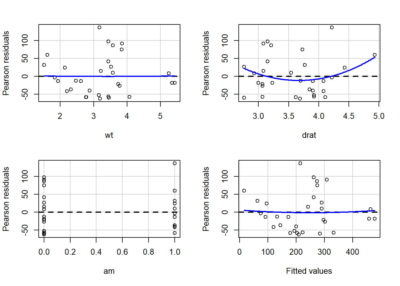

##            Test stat Pr(>|Test stat|)
## wt            0.0467           0.9631
## drat          1.3333           0.1936
## am           -0.1685           0.8675
## Tukey test    0.2071           0.8359

We see above that we received both some scatterplots as well as a table as output. Let’s start with an interpretation of the scatterplots. In the first few scatterplots, the regression residuals have been plotted against each independent variable, one at a time. These plots will help us test the assumption that residual errors are uncorrelated with all independent variables. These scatterplots have fit a blue line to the data. The scatterplot of residuals against wt show a flat line, meaning that the residuals are uncorrelated with wt. However, the scatterplot of residuals against drat shows a curved blue line, meaning that the residuals are not uncorrelated with the residuals. This problem—of drat being correlated with the residuals—is one that we would have to fix before we can trust the results. We will learn how to fix this problem in a later chapter in this textbook. Since am is a dummy variable, the computer does not draw a blue line. Based on our visual inspection, there does not appear to be any relationship between the residuals and the dummy variable am. Remember that if any one independent variable fails this diagnostic test, then the entire test fails and we cannot trust our results for inference.

Note that for our purposes, you can treat a Pearson residual as what we have been calling a residual or a residual error.

Based on our interpretation of the scatterplots above, we can start to fill out the diagnostic tests of assumptions checklist that we drafted earlier:

Completed?	Assumption	Result	Notes
	Residual errors have a mean of 0
	Residual errors are normally distributed
yes	Residual errors are uncorrelated with all independent variables	fail	`drat` failed; other independent variables passed
	All residuals are independent of (uncorrelated with) each other
	Homoscedasticity of residual errors
	Observations are independently and identically distributed
	Linearity of data
	No multicollinearity

Now we can turn to the final scatterplot that we received, which plots residuals against the predicted values (also called fitted values) of our dependent variable from the regression model reg1. This helps us test the linearity of data assumption. We again want the blue line to be flat, such that there is no relationship between the residuals and predicted values. In the plot above, we see that the blue line is almost flat but not quite. This is likely acceptable, but we will turn now to the output table that we received above to continue our diagnostic test of the linearity of data assumption.

In the output table that we received, we see a number of reported test statistics and p-values.¹³² As always, these p-values are the result of hypothesis tests. In this case, this is a “lack-of-fit”¹³³ hypothesis test to tell us if each variable is or is not well-fitted in our OLS regression model.

The hypothesis test for each independent variable is as follows:

$H_0$: The independent variable is linearly related to the dependent variable in the regression model.
$H_A$: The independent variable is non-linearly related to the dependent variable in the regression model.

The hypothesis test above has been conducted for us on each independent variable one at a time. Let’s practice interpreting the results. For wt, the p-value is 0.96, which is very high. This means that for wt, we did not find evidence for the alternate hypothesis that disp and wt are non-linearly related. Therefore, wt passes the test because we did not find any evidence to refute the null hypothesis that disp and wt are linearly related. Now we do the same evaluation for drat. The p-value for drat is 0.19, meaning that there is some limited support for the alternate hypothesis that disp and drat are non-linearly related. Given that we also saw a curved blue line in the scatterplot for drat, this might warrant further investigation, which you will learn how to do in a later chapter in this textbook. Finally, the test for am is also given but is not particularly meaningful since it is a dummy variable.

The very last row of the output table gives us the result of what is called “Tukey’s test for nonadditivity.”¹³⁴ In this case, the computer conducted a hypothesis test to determine if an alternate possible regression model (different from the OLS model we created) might be a better fit for the data.

Here is a summary of the hypotheses in Tukey’s test for nonadditivity:

$H_0$: Our regression model reg1 fits the data well (linearly, in this case).
$H_A$: A different regression model fits the data better.

To conduct this test, the computer created a different regression model behind the scenes. It then compared our regression model reg1 to this different behind-the-scenes model. The hypothesis test is to help us determine if a) our model reg1 is likely good enough or if b) the behind-the-scenes model is better in which case we should modify reg1. The p-value we received is 0.84, which is very high. This means that we did not find evidence for the alternate hypothesis. We can continue to cautiously assume the null hypothesis, since we did not find any evidence to the contrary from this test.

We are now ready to add to our checklist:

Completed?	Assumption	Result	Notes
	Residual errors have a mean of 0
	Residual errors are normally distributed
yes	Residual errors are uncorrelated with all independent variables	fail	`drat` failed; other independent variables passed
	All residuals are independent of (uncorrelated with) each other
	Homoscedasticity of residual errors
	Observations are independently and identically distributed
yes	Linearity of data	unclear	`drat` is ambiguous; other independent variables passed
	No multicollinearity

We found limited evidence of non-linearity for the independent variable drat. For all other variables and for the model overall, we did not find any other evidence of non-linearity. For the time being, we will note transparently and responsibly that the fit of the variable drat needs to be investigated further, but we will not conduct that further investigation. You will learn how to conduct this investigation in a future chapter.

9.1.3 Normality of residuals in R

The next set of diagnostic tests that we will do will test to see if our regression residuals are normally distributed. This tests the residual errors are normally distributed OLS assumption. We already learned how to test a distribution of data for normality when we tested our t-test samples for normality in a previous chapter. We will use the very same procedure to test our residuals for normality. Below, this entire process is demonstrated but with abbreviated commentary (because the detailed commentary would be exactly the same as the commentary you have already read in the t-test chapter).

Let’s begin by calculating the residuals of our regression model reg1. We already did this in the previous chapter but will do it again here as well.

This code will calculate the reg1 residuals and add them to our dataset d:

d$resid <- resid(reg1)

We will start by making a histogram of the residuals:

hist(d$resid)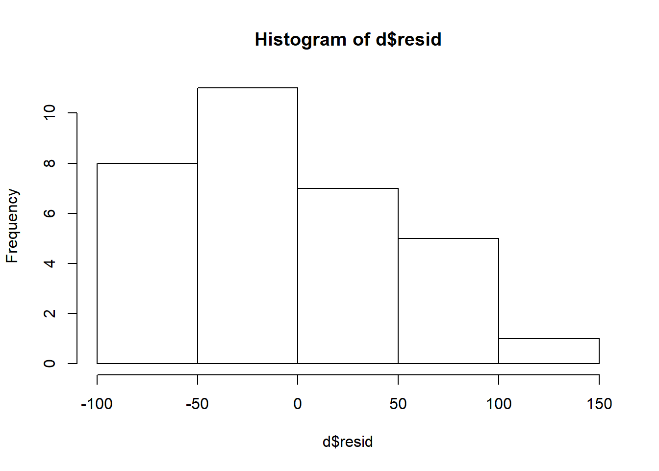

The histogram above follows a normally distributed pattern, but it is cut off on the left side. Preliminarily, this suggests that our residuals are not normally distributed.

Next, let’s make a QQ plot of our residuals:

if (!require(car)) install.packages('car')
library(car)

qqPlot(d$resid)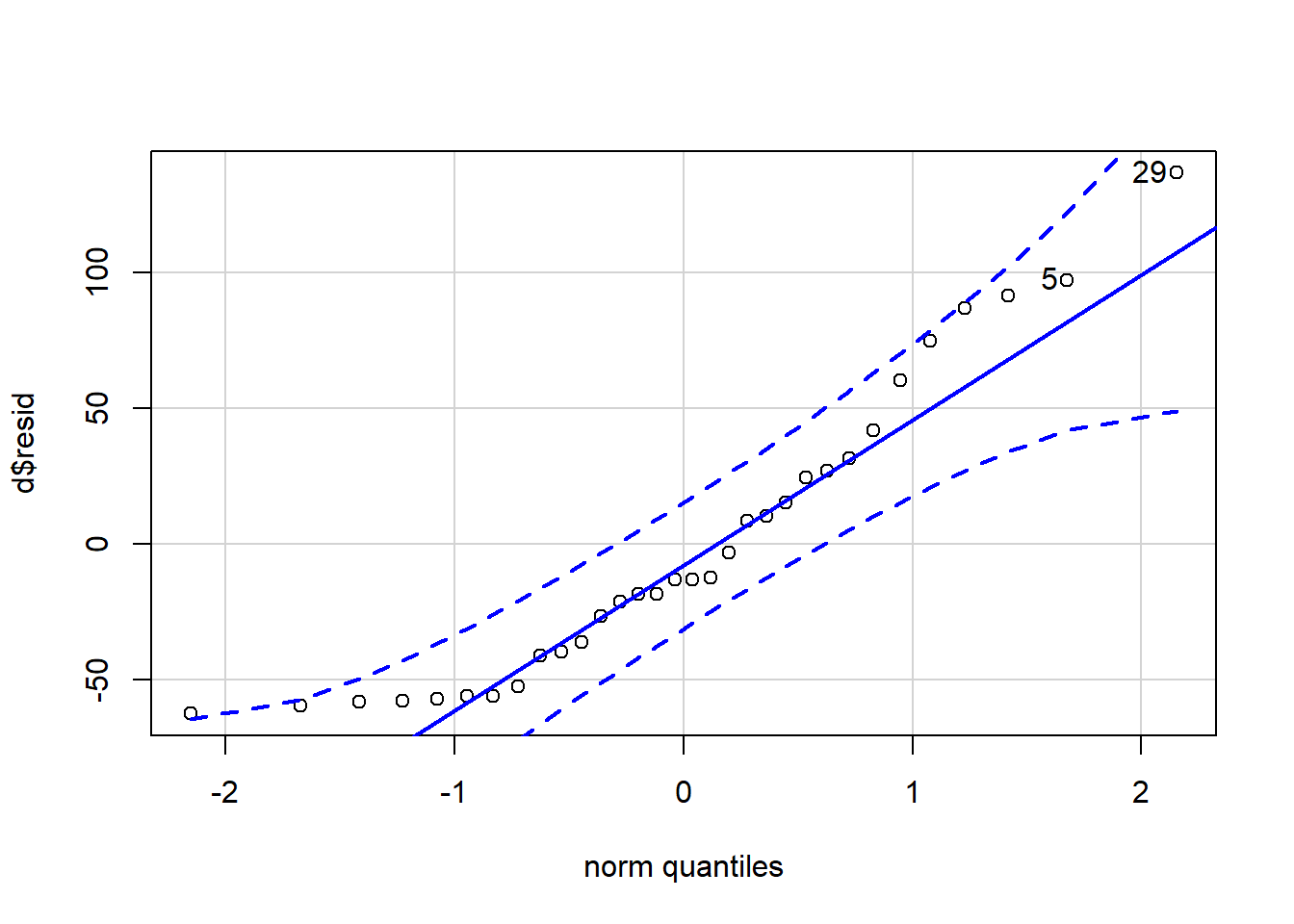

## [1] 29  5

Above, most of the points fall close to the blue line, indicating that they come from a normal distribution. But towards the extreme ends, some of the points start to deviate, with some even falling close to or going over the dotted confidence bands. Overall, this suggests that our data is likely normally distributed. However, we still might want to run our regression a second time after removing some of the observations that fall on the extreme ends of this distribution. Then we could compare the results of reg1 to those of our second regression and see if there are any differences.

Finally, we will conduct a Shapiro-Wilk test on our residuals using the code below:

shapiro.test(d$resid)

## 
##  Shapiro-Wilk normality test
## 
## data:  d$resid
## W = 0.90898, p-value = 0.01057

The extremely low p-value above tell us that our residuals are very likely not normally distributed. Therefore, we cannot trust the results of our OLS model for the purposes of inference.

Let’s continue to fill out our checklist now that we have tested the residuals of reg1 for normality:

Completed?	Assumption	Result	Notes
	Residual errors have a mean of 0
yes	Residual errors are normally distributed	fail
yes	Residual errors are uncorrelated with all independent variables	fail	`drat` failed; other independent variables passed
	All residuals are independent of (uncorrelated with) each other
	Homoscedasticity of residual errors
	Observations are independently and identically distributed
yes	Linearity of data	unclear	`drat` is ambiguous; other independent variables passed
	No multicollinearity

Our checklist is starting to fill out. Let’s keep going, below!

9.1.4 Autocorrelation of residuals in R

We will now test the OLS assumption that all residuals are independent of (uncorrelated with) each other. When we conduct this diagnostic test, we will be testing for what is called autocorrelation. To do this, we will do one visual test and one hypothesis test.

To conduct the visual test, we will look at a scatterplot of the residuals plotted against the row number of each observation, which can be generated using the code below:

plot(seq(1:nrow(d)),d$resid, )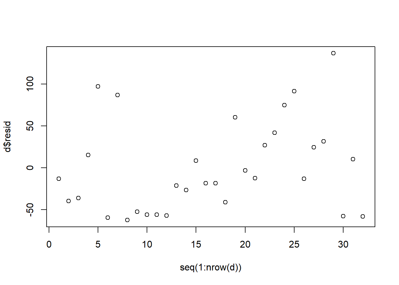

Before we interpret the code above, let’s review what the code we used did:

plot(...) – We want to make a scatterplot.
seq(1:nrow(d)) – This is the first argument we gave to the plot(...) function. This is what will be plotted on the horizontal axis of the scatterplot. What we wanted on the horizontal axis of the scatterplot is simply the row number of each observation. To generate the row numbers as a variable to give to the plot(...) function, we used the seq(...) function. The seq(...) function creates a variable that is a sequence. In this case, we asked it to create a sequence for us from 1 up to the number of rows in the dataset d, which we calculated with the nrow(...) function. We put the nrow(...) function within the seq(...) function within the plot(...) function. To use this code on your own, you can replace d with the name of your own dataset.
d$resid – This is the second argument that we gave to the plot(...) function. This means that we want the variable resid that is within the dataset d to be plotted on the vertical axis of the scatterplot.

In the scatterplot that we received, we are looking for any noticeable pattern in the residuals. Ideally, we would just see complete randomness, with no relationship between residuals that are adjacent to each other. For the most part, we do see fairly random residuals, especially on the right half of the plot (observation 13 and above). However, if we look closely, we also see that observations 8–12 all appear to have almost the same residual. You can find these by looking in the scatterplot where there is a row of points that all have a residual of approximately -50 (on the vertical axis) and row numbers (on the horizontal axis) between 8 and 12. This is evidence of autocorrelation and might be a problem. Let’s dig deeper, below.

Here is a table with our dataset d and all of the variables that are involved in our analysis:

d[c("disp","wt","drat","am","resid")]

##                      disp    wt drat am      resid
## Mazda RX4           160.0 2.620 3.90  1 -13.047902
## Mazda RX4 Wag       160.0 2.875 3.90  1 -39.774061
## Datsun 710          108.0 2.320 3.85  1 -36.142749
## Hornet 4 Drive      258.0 3.215 3.08  0  15.203849
## Hornet Sportabout   360.0 3.440 3.15  0  97.174286
## Valiant             225.0 3.460 2.76  0 -59.713506
## Duster 360          360.0 3.570 3.21  0  86.594051
## Merc 240D           146.7 3.190 3.69  0 -62.519811
## Merc 230            140.8 3.150 3.92  0 -52.555489
## Merc 280            167.6 3.440 3.92  0 -56.149945
## Merc 280C           167.6 3.440 3.92  0 -56.149945
## Merc 450SE          275.8 4.070 3.07  0 -57.114869
## Merc 450SL          275.8 3.730 3.07  0 -21.479990
## Merc 450SLC         275.8 3.780 3.07  0 -26.720413
## Cadillac Fleetwood  472.0 5.250 2.93  0   8.306454
## Lincoln Continental 460.0 5.424 3.00  0 -18.377877
## Chrysler Imperial   440.0 5.345 3.23  0 -18.426025
## Fiat 128             78.7 2.200 4.08  1 -41.193750
## Honda Civic          75.7 1.615 4.93  1  60.254793
## Toyota Corolla       71.1 1.835 4.22  1  -3.433974
## Toyota Corona       120.1 2.465 3.70  0 -12.626194
## Dodge Challenger    318.0 3.520 2.76  0  26.997986
## AMC Javelin         304.0 3.435 3.15  0  41.698329
## Camaro Z28          350.0 3.840 3.73  0  74.684595
## Pontiac Firebird    400.0 3.845 3.08  0  91.174514
## Fiat X1-9            79.0 1.935 4.08  1 -13.119506
## Porsche 914-2       120.3 2.140 4.43  1  24.456471
## Lotus Europa         95.1 1.513 3.77  1  31.477865
## Ford Pantera L      351.0 3.170 4.22  1 136.546721
## Ferrari Dino        145.0 2.770 3.62  1 -57.978543
## Maserati Bora       301.0 3.570 3.54  1  10.114863
## Volvo 142E          121.0 2.780 4.11  1 -58.160229

Above, if we count down to the 8th, 9th, 10th, 11th, and 12th rows, we see that all of those cars are Merc cars. And all of them have a residual of approximately -50. This is unacceptable. This means that there is non-randomness in our residuals. This means that we should not necessarily trust our OLS results for the purposes of inference. This also uncovers a potential problem with our research design. What population does this sample represent? Can we reasonably say that this sample represents all cars? Probably not. When we do inference, we have to be mindful not only of the diagnostic tests that we do in R but also of how our research design and sampling strategy might influence our results.

Anyway, with some possible visual evidence of autocorrelation in mind, let’s turn to a hypothesis test that can help us further investigate. We will run the Durbin-Watson test for autocorrelation.

Here are the hypotheses for the Durbin-Watson test:

$H_0$: Residuals are not autocorrelated.
$H_A$: Residuals are autocorrelated.

And here is how we run the Durbin-Watson test in R:

if (!require(lmtest)) install.packages('lmtest')
library(lmtest)

dwtest(reg1)

## 
##  Durbin-Watson test
## 
## data:  reg1
## DW = 1.8701, p-value = 0.2462
## alternative hypothesis: true autocorrelation is greater than 0

In the code we ran above, we first installed the lmtest package if necessary, loaded the lmtest package, and then ran the dwtest(...) function with our regression model reg1 as an argument in that function. This ran the hypothesis test for us.

The resulting p-value of 0.25. Is not strong enough to worry us about autocorrelation as a result of the Durbin-Watson test in and of itself. Of course, since we found visual and theoretical evidence of possible autocorrelation due to the Merc observations, we will still consider our OLS model reg1 to have failed the autocorrelation diagnostic test.

Let’s add to our OLS diagnostics checklist:

Completed?	Assumption	Result	Notes
	Residual errors have a mean of 0
yes	Residual errors are normally distributed	fail
yes	Residual errors are uncorrelated with all independent variables	fail	`drat` failed; other independent variables passed
yes	All residuals are independent of (uncorrelated with) each other	fail
	Homoscedasticity of residual errors
	Observations are independently and identically distributed
yes	Linearity of data	unclear	`drat` is ambiguous; other independent variables passed
	No multicollinearity

Before we conclude our study of autocorrelated residuals, let’s see an extreme example of what problematic autocorrelation would look like. Have a look at the scatterplot below of hypothetical residuals plotted against hypothetical observations, from another hypothetical regression.

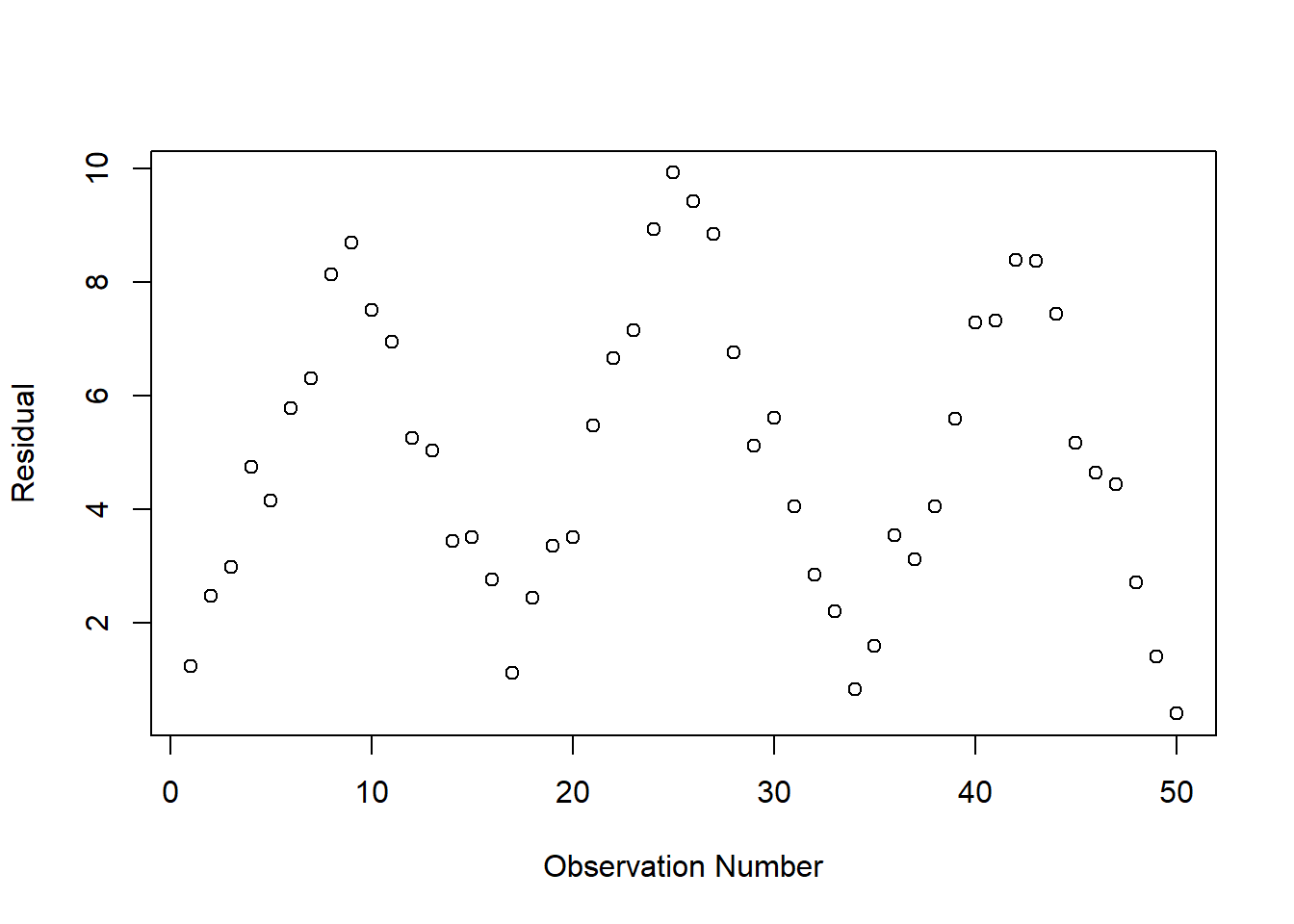
Above is an example of extreme autocorrelation. Each observation’s residual is very close to the residual of the previous observation. The residuals are not random at all. Each residual is likely related to the residual before and after it. Residuals that appear like this indicate a potential problem that require further investigation.

9.1.5 Homoscedasticity of residuals in R

Another OLS assumption is homoscedasticity of residual errors. The diagnostic tests for this assumption are also conducted both as a visual examination and a hypothesis test. We will begin with a visual test. We will conduct this visual test by looking at a scatterplot that we have already seen once before: the plot of the residuals plotted against the predicted values. This was part of the output that we received when we ran the residualPlots(...) command earlier in the chapter.

Here is a copy of the residuals plotted against predicted values, so that you don’t have to go up to look at it again:

if (!require(car)) install.packages('car')
library(car)

residualPlots(reg1, ~1, fitted=TRUE)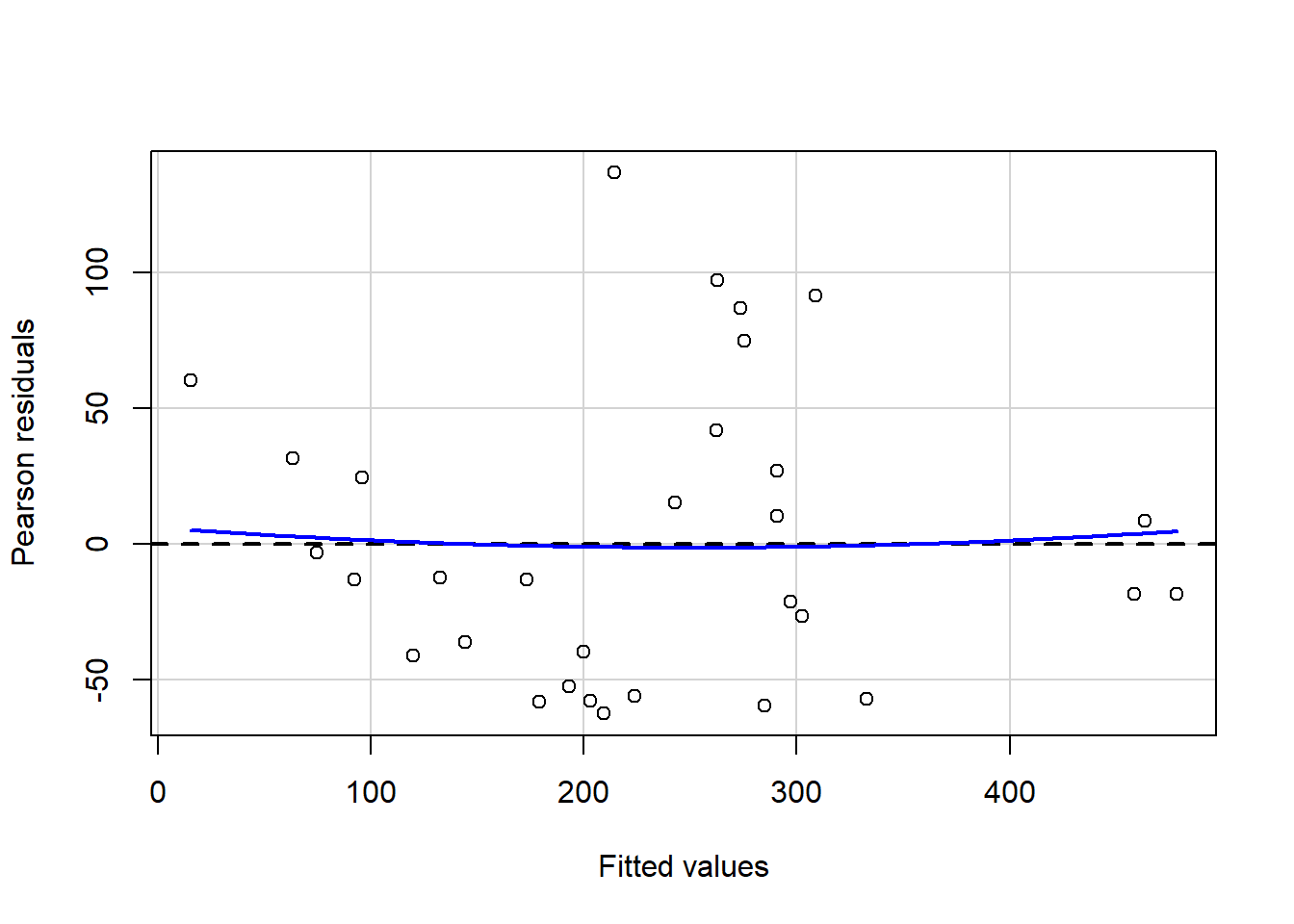

##            Test stat Pr(>|Test stat|)
## Tukey test    0.2071           0.8359

This time, we are looking in the scatterplot above to see if there is any noticeable pattern in the variance—or spread—of the residuals. Ideally, we would see complete randomness, with the residuals spread out fairly evenly around the horizontal black dotted line as we look across the scatterplot horizontally. This would indicate that the residuals are evenly distributed. If we instead see a noticeable pattern in the residuals across the predicted values, that would indicate a problem. In this case there does not appear to be any kind of pattern. So far, we can probably safely assume that our residuals are homoscedastic, meaning that they have constant variance. If we had noticed a pattern, then we would instead refer to our residuals as heteroscedastic, which would be a violation of the OLS assumptions.

Let’s turn to the hypothesis test of homoscedasticity. This is called the Breusch-Pagan test. For the Breusch-Pagan test, we have the following hypotheses:

$H_0$: The variance of the residuals is constant. The residuals are homoscedastic.
$H_A$: The variance of the residuals is not constant. The residuals are heteroscedastic.

if (!require(car)) install.packages('car')
library(car)

ncvTest(reg1)

## Non-constant Variance Score Test 
## Variance formula: ~ fitted.values 
## Chisquare = 0.005343423, Df = 1, p = 0.94173

Above, we yet again loaded the car package first. We then ran the ncvTest(...) function with our regression model reg1 as the argument within that function. This code conducted a Breusch-Pagan test.

The p-value of 0.94 shows that there is no evidence of heteroscedasticity in our regression model reg1. Since both visual inspection and the Breusch-Pagan test did not show any evidence of heteroscedasticity, we can conclude that our model reg1 passes this diagnostic test and does not violate the OLS assumption of homoscedasticity of residual errors.

Let’s add this diagnostic test result to our checklist:

Completed?	Assumption	Result	Notes
	Residual errors have a mean of 0
yes	Residual errors are normally distributed	fail
yes	Residual errors are uncorrelated with all independent variables	fail	`drat` failed; other independent variables passed
yes	All residuals are independent of (uncorrelated with) each other	fail
yes	Homoscedasticity of residual errors	pass
	Observations are independently and identically distributed
yes	Linearity of data	unclear	`drat` is ambiguous; other independent variables passed
	No multicollinearity

Before we conclude our examination of homoscedasticity, let’s look at an example of what clear heteroscedasticity would look like. Have a look at the example scatterplot below of hypothetical residuals plotted against hypothetical predicted values from a hypothetical regression model.

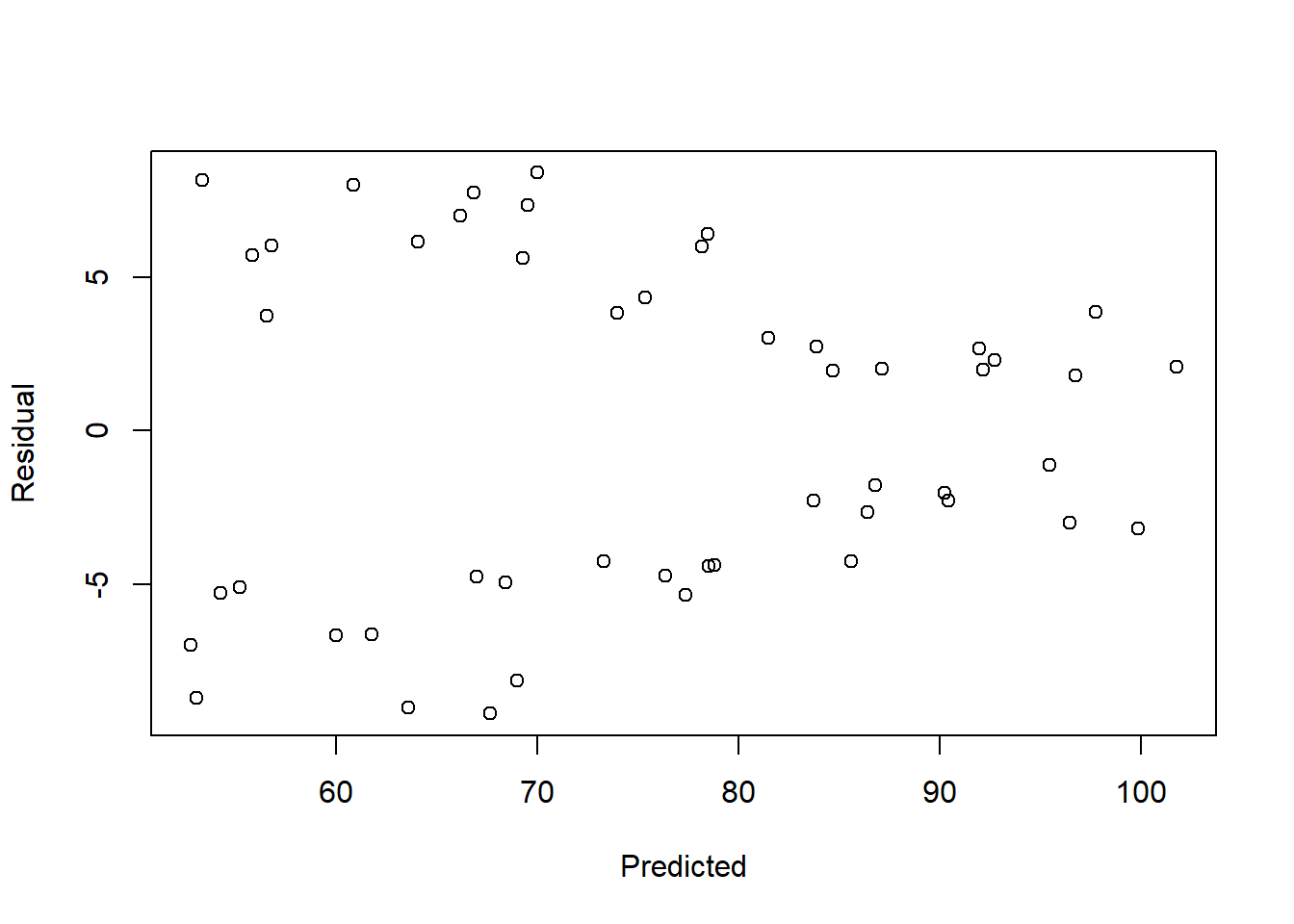
Above, we see that the residuals fall into what we could call a cone shape. The wide base of the cone is on the left and the narrow top of the cone is on the right. The variance—or spread—of the residuals is large at low predicted values (on the left side of the plot) and small at higher predicted values (on the right side of the plot). If we had found residuals like we see in the plot above, we would conclude that our residuals are heteroscedastic. A regression model with heteroscedastic residuals violates the homoscedasticity OLS assumption and cannot be trusted for inference.

9.1.6 Multicollinearity detection in R

Now it is time to discuss an OLS assumption that does not relate to the residuals: no multicollinearity. Multicollinearity is a diagnostic test that relates only to the independent variables in a regression model. Multicollinearity is a problem that occurs in an OLS model when the independent variables are too highly correlated with each other. Testing for multicollinearity has nothing to do with the dependent variable or the residuals of a regression model.

The first step is to simply look at the correlation of the independent variables in our regression models. One way to do this is to make a copy of our dataset d called d.partial that only contains our three independent variables.

Below, we create d.partial with only our three independent variables wt, drat, and am:

d.partial <- d[c("wt","drat", "am")]

Next, we can run the same cor(...) function that we have used before, but this time with our dataset d.partial as the function’s only argument:

cor(d.partial)

##              wt       drat         am
## wt    1.0000000 -0.7124406 -0.6924953
## drat -0.7124406  1.0000000  0.7127111
## am   -0.6924953  0.7127111  1.0000000

Above, the computer created a correlation matrix for us. It calculated the correlation of each variable in the dataset d.partial with every other variable in the dataset. For example, we see that wt and drat are correlated with each other at -0.71.

We can also once again create a fancier version of this correlation matrix:

if (!require(PerformanceAnalytics)) install.packages('PerformanceAnalytics')
library(PerformanceAnalytics)

chart.Correlation(d.partial, histogram = TRUE)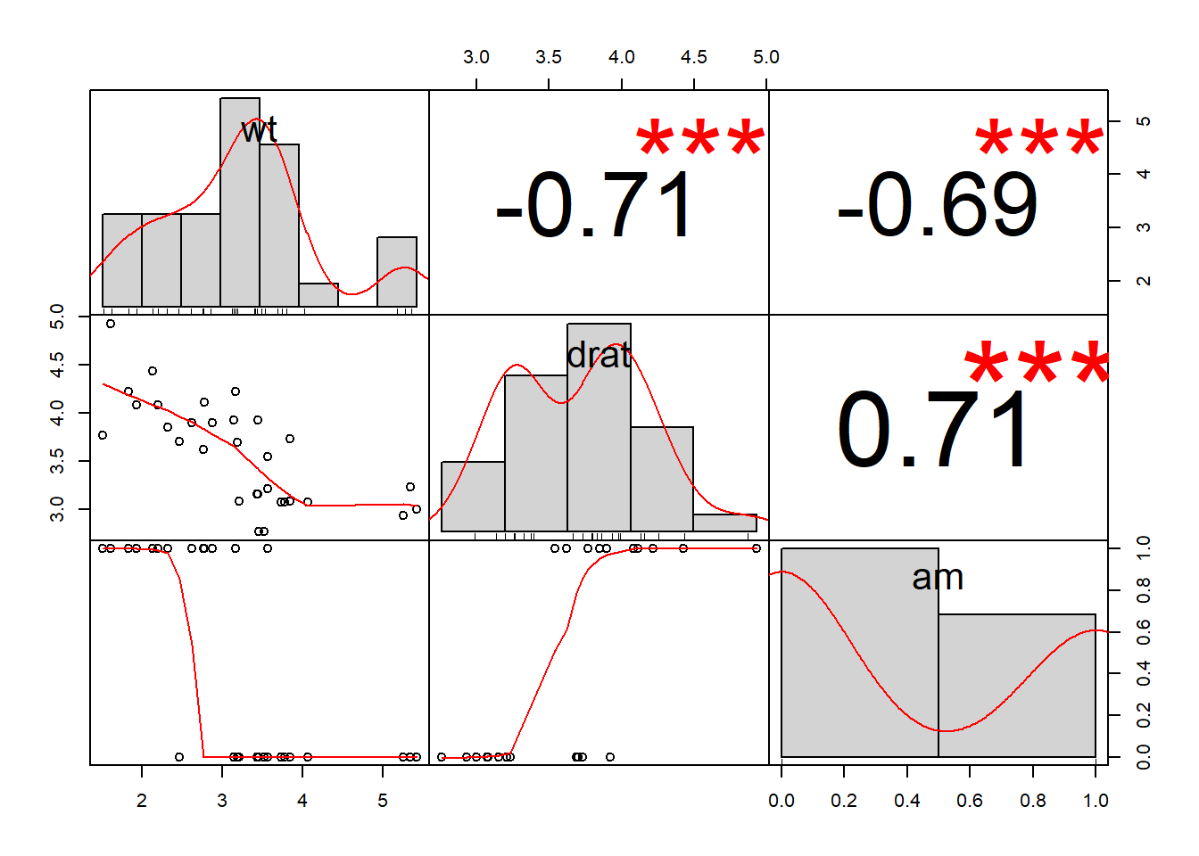

Now that we have generated both plain and fancy versions of our correlation matrix, let’s get down to analyzing this output to check for multicollinearity. When the problem of multicollinearity is present, that means that the independent variables are too highly correlated with each other. The problem of multicollinearity can cause the hypothesis test for each slope calculation in the OLS regression to be conducted incorrectly. When multicollinearity is a present, the p-value and confidence interval for each slope estimate may not be trustworthy. In the correlation matrix above, all of the variables are highly correlated with each other. Remember: the maximum amount of correlation possible is either -1 or +1. -1 is a very high negative correlation and +1 is a very high positive correlation. The correlations we see above are all very close to either -1 or +1, meaning that multicollinearity may be a problem in our regression model reg1.

In the example above, all of the independent variables are highly correlated with each other. However, note that even if any two independent variables are highly correlated with each other, that is cause for concern and you should consider removing one of those independent variables from the regression model, if possible.

The next way to test for multicollinearity is by looking at the VIF—variance inflation factor—of each independent variable in our OLS regression model.

Here is the code we use to do the VIF test:

if (!require(car)) install.packages('car')
library(car)

vif(reg1)

##       wt     drat       am 
## 2.363655 2.500118 2.365507

In the code above, we loaded the car package and then ran the vif(...) function with reg1 as the function’s argument. The computer then gave us VIF values for each independent variable. Note that these are not p-values or confidence intervals. These are something different. They are VIF values.

When a variable has a VIF value of 4 or more, that indicates that multicollinearity might be a problem in our regression model. All of these VIF values are under 4, so we can say that our OLS model reg1 passes the VIF test. However, we cannot ignore the very high correlation of the independent variables that we saw earlier. Typically, such high correlations would be too high and we would adjust our regression model by removing one or more independent variables and running it again. There are also more complicated methods that can be used to resolve multicollinearity, but these are beyond the scope of this textbook.

Any time you find high correlations among any two or more independent variables or high VIF values, you should first try removing an independent variable from your regression model and running the regression again. There are also other, more advanced ways to fix multicollinearity which do not involve removing one or more variables from your regression model.¹³⁵ Often, these more advanced approaches are not necessary. These approaches are beyond the scope of this textbook.

We are now ready to add our result of the no multicollinearity OLS diagnostic test to our checklist:

Completed?	Assumption	Result	Notes
	Residual errors have a mean of 0
yes	Residual errors are normally distributed	fail
yes	Residual errors are uncorrelated with all independent variables	fail	`drat` failed; other independent variables passed
yes	All residuals are independent of (uncorrelated with) each other	fail
yes	Homoscedasticity of residual errors	pass
	Observations are independently and identically distributed
yes	Linearity of data	unclear	`drat` is ambiguous; other independent variables passed
yes	No multicollinearity	unclear	VIF passed but correlations are very high

9.1.7 Mean of residuals

Another OLS assumption is that the residual errors have a mean of 0. We already calculated the residuals of our regression model reg1 and added them to our dataset d as the variable resid. So, let’s just go ahead and see what the mean of these residuals is.

This code calculates the mean of the reg1 residuals:

mean(d$resid)

## [1] -1.554312e-15

Above, we see that the mean of the residuals is an extremely small number. This is basically 0. In fact, in OLS, the mean of the residuals of our regression model is always 0. That is how OLS linear regression is programmed. The math used to calculate OLS linear regression results require that the mean of the residuals is 0. Therefore, this is not an assumption that we can test. As you read earlier, the residual errors should have a population mean of 0.¹³⁶ This means that our test of this assumption is more theoretical than anything else. We have to ask ourselves: is there anything about our sampling method, the population from which we are sampling, our research design as a whole, or any other factor that might cause our regression residuals to be non-random? If the regression residuals are random, their population mean will be 0. If something is causing the residuals to be non-random, then the population mean of the residuals may not be random and the OLS assumption that the residual errors have a mean of 0 would be violated and we could not trust our regression results to conduct inference.

For now, since we do not know much about how the cars in our dataset were sampled, let’s conclude that we don’t know for sure if the population mean of our residuals is 0 or not. That is what we will write into our checklist.

Here is an updated copy of our checklist:

Completed?	Assumption	Result	Notes
yes	Residual errors have a mean of 0	unclear	Inadequate information about research design
yes	Residual errors are normally distributed	fail
yes	Residual errors are uncorrelated with all independent variables	fail	`drat` failed; other independent variables passed
yes	All residuals are independent of (uncorrelated with) each other	fail
yes	Homoscedasticity of residual errors	pass
	Observations are independently and identically distributed
yes	Linearity of data	unclear	`drat` is ambiguous; other independent variables passed
yes	No multicollinearity	unclear	VIF passed but correlations are very high

9.1.8 Independence of observations

Only one diagnostic test remains, the test of the OLS assumption that observations are independently and identically distributed (this is often called the “IID” assumption). We will use our knowledge of theory and research design to test this assumption. To satisfy this assumption and pass this diagnostic test, observations in our data should not influence each other in any way or have measurable characteristics that are related to each other in any way. For example, if we are sampling 100 people to test how well they do on a test, if some students work together in groups instead of working alone to answer the test questions, their results are not independent of each other. Students who worked in groups together influenced each other’s results.

In our example analysis for which we created the OLS regression model reg1, we do not have sufficient knowledge about how the observations in our dataset d were selected. If they were selected non-randomly, then we likely violate the IID assumption. Typically, if we have a reliable sampling strategy that randomly samples observations into a dataset from the population of interest, we will satisfy the IID assumption of OLS.

For now, we will complete our checklist in a way that reflects our uncertainty about the IID assumption for reg1:

Completed?	Assumption	Result	Notes
yes	Residual errors have a mean of 0	unclear	Inadequate information about research design
yes	Residual errors are normally distributed	fail
yes	Residual errors are uncorrelated with all independent variables	fail	`drat` failed; other independent variables passed
yes	All residuals are independent of (uncorrelated with) each other	fail
yes	Homoscedasticity of residual errors	pass
yes	Observations are independently and identically distributed	unclear	Inadequate information about research design
yes	Linearity of data	unclear	`drat` is ambiguous; other independent variables passed
yes	No multicollinearity	unclear	VIF passed but correlations are very high

It is important to make sure that your research design is appropriate for the question you are trying to answer. If the question you are trying to answer will be answered using an OLS regression model that analyzes a sample to make an inference about a population, your research/project design should be such that the IID assumption of OLS is definitely satisfied. You should also try to maximize the chances that most other OLS assumptions will also be satisfied. Of course, this might not always be possible. A large portion of the remainder of this textbook is devoted to creating regression models that are more appropriate than OLS linear regression for situations in which our research design and/or data violate the OLS assumptions and fail to pass the diagnostic tests that we have just reviewed.

9.1.9 Conclusion of diagnostic testing

We have now completed all of the diagnostic tests of OLS assumptions that must be conducted before an OLS regression result can be trusted for the purposes of inference. As you practice, you will become more and more used to conducting these tests after every regression model you run. It may seem like a lot of tests now, but if you repeat these tests on many different datasets and regression models, you will develop speed and comfort. You will also develop your own library of R commands that you save within your own RMarkdown files that you can quickly find and modify each time you work on a new project. This is why it is important for all of your quantitative analysis work to be saved carefully and coded in a reproducible way.

In the example presented in this chapter, our regression model reg1 failed most of the diagnostic tests. Therefore, it would be irresponsible for us to make claims about an entire population of automobiles based on this sample of 32 automobiles. Our regression results do tell us on average what is happening within our sample alone, but they do not tell us anything trustworthy about a population.

Finally, one topic that is not discussed in this chapter is analysis of outliers. The presence of outliers in our data may sometimes cause our regression model to violate some of the OLS regression assumptions. Sometimes, only if it is reasonable to do so, we can remove one or more outliers from our data before running a regression. The most responsible thing to do is to run our regression with and without any outliers and see if we get the same results both times. If we do get similar results each time, we can be more confident about our results. If we do not get similar results each time, we should hesitate to make a definitive conclusion and instead report exactly what happened (that we got conflicting or inconclusive results). Alternatively, if we do not get similar results each time, we should have a strong justification for choosing one regression result over another.

There are many techniques can be used to identify outliers. However, outlier identification is beyond the scope of this chapter.

9.2 Summary of regression research process

In general, the overall process we should follow when using OLS and other regression methods to do research or a project is:

Ask a question that we want to answer using numbers.
Gather and/or prepare the appropriate data to answer the question.
Run the appropriate regression model.
Examine goodness-of-fit.
Run diagnostic tests of regression model assumptions to determine if we can or cannot trust our regression results.
Make any necessary modifications to data and/or regression model specification and then repeat steps above as many times as necessary.
If goodness-of-fit and diagnistic tests results are satisfactory, carefully interpret regression results and cautiously make conclusions.
Transparently report the entire process and results.

9.3 Dummy variables

“Dummy” variables are variables that just have two values. Here are some examples:

Variable	Levels
gender	female, male
experimental group	treatment, control
completed training	did complete training, did not complete training
citizenship	native, foreign
test result	pass, fail
transmission type	automatic, manual

How does this look within a dataset? Maybe you would have a variable in your dataset called gender and it would be coded as 1 for females and 0 for males. Note that constructs like gender are qualitative. Male and female are not numeric concepts. By converting them into 1 and 0, we made them numeric. This is analogous to how we incorporated and interpreted the am variable in our reg1 example.

A dummy variable can also be called a binary variable, dichotomous variable, yes/no variable, two-level categorical variable, or anything similar. All of these terms mean the same thing.

But what about when you have three or more qualitative (non-numeric) categories that you want to include in your regression as a single variable?

Here are some examples:

Variable	Levels
Race	black, white, other
Favorite ice cream flavor	chocolate, vanilla, strawberry, other
Type of car owned	Gas, electric, hybrid, do not have a car

Let’s add a qualitative variable with three or more categories to the dataset d—which is a copy of mtcars—that we were using earlier. We will call this new variable region, to indicate what part of the world a car was made in.

Here, we add the region variable to d:

d$region <- c("asia","asia","asia","northamerica","northamerica","northamerica","northamerica","europe","europe","europe","europe","europe","europe","europe","northamerica","northamerica","northamerica","europe","asia","asia","asia","northamerica","northamerica","northamerica","northamerica","europe","europe","europe","northamerica","europe","europe","europe")

Now the dataset d has a new variable called region. The variable region has three levels: asia, northamerica, and europe. region is a categorical variable. How can we possibly analyze it quantitatively?

Well, one option is to make a boxplot:

boxplot(disp ~ region, data = d)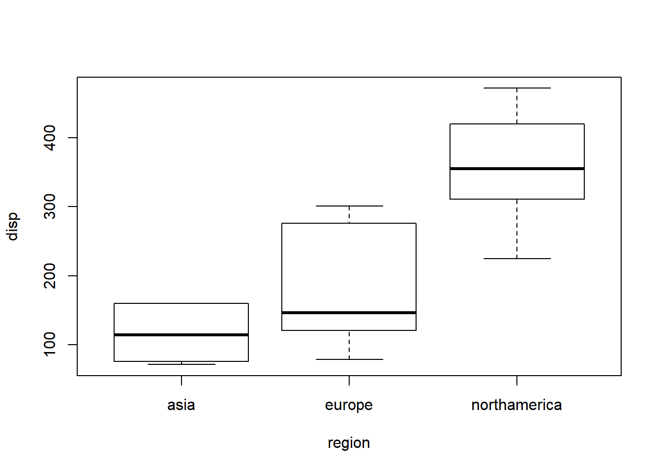

Above, we see that disp, our dependent variable of interest, seems to be quite different across cars from the three different regions. Now we want to examine this relationship in a regression analysis where we can control for other variables. Let’s set up our research design.

Research design:

Question of interest: Does displacement differ in cars from different regions?
Data: copy of mtcars data called d
Analytic method: OLS
Dependent variable: disp
Independent variables: wt, drat, am, region

We are almost ready to run a regression. We know what question we want to answer, we have our data and variables. But one variable—region—is not numeric. How can we make it numeric so that we can put it into our OLS regression? We will have to create multiple dummy variables to help identify each observation.

The code below creates dummy variables for us for the variable d$region:

if (!require(fastDummies)) install.packages('fastDummies')
library(fastDummies)

d <- dummy_cols(d,select_columns = c("region"))

Here’s what the code above did:

Load fastDummies package. This is a package that is specifically designed to help us quickly turn a qualitative categorical variable like region into dummy variables.
d <- – Replace the dataset d with a new version of d that is created by the dummy_cols(...) function.
dummy_cols(d,select_columns = c("region")) - Run the dummy_cols(...) function which will turn a categorical variable into multiple dummy variables. This function has two arguments:
- d – This is the dataset that is being used.
- select_columns = c("region") – This tells the computer which variables in the original dataset d we want to turn into dummy variables. In this case, region is the only one we have specified, but we could add others too if we wanted.

Let’s inspect the new version of d. You can do this by running View(d) on your computer. Three new dummy variables were generated, called region_europe, region_asia, and region_northamerica.

Below is an example of three observations (cars) selected from the data, one from each region:

region	region_europe	region_asia	region_northamerica
northamerica	0	0	1
europe	1	0	0
asia	0	1	0

Let’s go through an example: The first car is from North America. Its region, the qualitative variable, was coded as northamerica. In our three dummy variables, it is coded as 0 for region_europe and region_asia. It is coded as 1 for region_northamerica.

Now let’s remove the first column from the table:

region_europe	region_asia	region_northamerica
0	0	1
1	0	0
0	1	0

Using just the dummy variables in the table above, we can tell that the first car is from North America, the second car is from Europe, and the third car is from Asia. And now we are doing it all using numbers and all using variables that are coded as either 0 or 1! We turned the qualitative categorical variable region, which had three levels, into three dummy variables which each have two levels (0 and 1).

Now we can make a regression model to answer our question:¹³⁷

reg2 <-  lm(disp~wt+drat+am+region_europe+region_asia, data = d)

Above, we made a regression model that we saved as reg2. The dependent variable is disp. The independent variables are wt, drat, am, region_europe, and region_asia. Note that we left out region_northamerica from the list of independent variables. You always have to leave out one dummy variable from the regression for any particular qualitative categorical variable. In this case, the qualitative categorical variable region led to the creation of three dummy variables; one of those dummy variables must be left out of the regression. The category that is left out of the regression is called the reference category. Above, North American cars are the reference category. Let’s have a look at our regression results:

if (!require(jtools)) install.packages('jtools')
library(jtools)

summ(reg2, confint = TRUE)

Observations	32
Dependent variable	disp
Type	OLS linear regression

F(5,26)	59.98
R²	0.92
Adj. R²	0.90

	Est.	2.5%	97.5%	t val.	p
(Intercept)	69.47	-120.37	259.31	0.75	0.46
wt	86.18	62.83	109.53	7.59	0.00
drat	-17.49	-60.96	25.99	-0.83	0.42
am	39.53	-4.14	83.19	1.86	0.07
region_europe	-109.92	-147.60	-72.24	-6.00	0.00
region_asia	-112.38	-165.86	-58.91	-4.32	0.00
Standard errors: OLS

The equation for this regression model is:

\[\hat{y} = 86.18wt - 17.49drat + 39.53am -109.92region\text{_}europe -112.38region\text{_}asia + 69.47\]

The predicted value of disp for a car that weighs 1.5 tons, has a rear axle ratio of 2 units, has an automatic transmission, and was made in Asia would be calculated like this:

$\hat{y} = (86.18*1.5) - (17.49*2) + (39.53*0) - (109.92*0) -(112.38*1) + 69.47 = 51.38 \text{ cubic inches}$

If this same car was instead made in North America, we would calculate its predicted disp like this:

$\hat{y} = (86.18*1.5) - (17.49*2) + (39.53*0) - (109.92*0) -(112.38*0) + 69.47 = 163.76 \text{ cubic inches}$

In this regression model, we would interpret wt, drat, and am the same way we did earlier in the chapter. Let’s focus just on our two new dummy variables, region_europe and region_asia.

Interpretation of region dummy variables, in our sample:

Cars that are made in Europe are predicted on average to have displacement that is 109.92 cubic inches lower than displacement of cars made in North America, controlling for all other independent variables.
Cars that are made in Asia are predicted on average to have displacement that is 112.38 cubic inches lower than displacement of cars made in North America, controlling for all other independent variables.

Interpretation of region dummy variables, in the population from which our sample was drawn:

We are 95% confident that cars that are made in Europe have on average a displacement that is between 147.60 and 72.24 cubic inches lower than displacement of cars made in North America, controlling for all other independent variables.
We are 95% confident that cars that are made in Asia have on average a displacement that is between 165.86 and 58.91 cubic inches lower than displacement of cars made in North America, controlling for all other independent variables.
These results are of course only trustworthy if our model and data pass all diagnostic tests and satisfy all OLS assumptions.

Importantly, notice that the regression results for these region dummy variables can only tell us how European and Asian cars compare to North American cars. They can NOT tell us how European and Asian cars compare to each other. This is because we decided to leave out the North American cars dummy variable from the regression and designate it as the reference category. If we had wanted, we could have left out one of the other regions as the reference category. if we had left Europe out of the regression and we had included Asia and North America, then we would be comparing the displacement of Asian and North American cars to that of European cars.

You might be wondering: Why can’t we just include all three dummy variables in the regression? The reason we cannot do this is because doing so would violate at least one OLS regression assumption. We cannot include variables that are perfect linear combinations of each other. In fact, the computer would not even allow you to do so. It would remove one of the three variables for you from the regression model. One way to think about it is like this: Once the computer knows whether a car is Asian or not and it also knows if that car is European or not, it definitely knows already if that car is North American or not. You don’t need to explicitly tell the computer. Therefore, just two of the dummy variables are enough for the computer to know everything about your data related to the region variable. Adding in the third dummy variable would be redundant, unnecessary information.

In all cases, we include one dummy variable fewer than the number of categories in the qualitative categorical variable that we are trying to analyze:

\[number\; of\; dummy\; variables = number\; of\; categories - 1\]

Also, keep in mind that the computer “thinks” that the variables region_asia and region_europe are continuous numeric variables. It does not know that these variables can only have a value of 0 or 1. The same is the case for the am variable, as we discussed earlier in the chapter.

As you continue to learn more about quantitative analysis, you are likely to run into situations where you need to do quantitative analysis on qualitative data. The strategy of dividing qualitative categorical data into dummy variables can be very handy and it is a good skill to practice. We will be using dummy variables repeatedly in the rest of this textbook for a variety of useful purposes.

9.4 Assignment

In this chapter’s assignment, you will continue the work you did in the previous assignment. Please find and re-run the regression model you made in the previous chapter—the one that used the hsb2 dataset—in preparation for the assignment below.

9.4.1 OLS regression with dummy variables

Task 1: Create dummy variables for the variables gender and prog (from the hsb2 dataset) in preparation for adding them to the regression model. Show all of the code you used to create these dummy variables.

Task 2: Re-run your regression model from the previous chapter, with gender and prog dummy variables added. Interpret the results for both sample and population.

9.4.2 Diagnostic tests of OLS assumptions

Now you will run and interpret all required diagnostic tests for the OLS regression model that you created earlier in the assignment.

Task 3: Make an empty checklist of the OLS diagnostic tests on a piece of paper, so that you can check off tests as you do them.¹³⁸ You do not need to submit this checklist.

Task 4: Conduct and show/explain the results of ALL diagnostic tests for multiple OLS. Your answer to this task will likely be quite long and have multiple sections.

9.4.3 Follow up and submission

You have now reached the end of this week’s assignment. The tasks below will guide you through submission of the assignment and allow us to gather questions and/or feedback from you.

Task 5: Please write any questions you have for the course instructors (optional).

Task 6: Please write any feedback you have about the instructional materials (optional).

Task 7: Please e-mail Nicole and Anshul to schedule Oral Exam #2 if you have not done so already.

Task 8: Knit (export) your RMarkdown file into a format of your choosing.

Task 9: Please submit your assignment to the D2L assignment drop-box corresponding to this chapter and week of the course. And remember that if you have trouble getting your RMarkdown file to knit, you can submit your RMarkdown file itself. You can also submit an additional file(s) if needed.

Frost, Jim. “7 Classical Assumptions of Ordinary Least Squares (OLS) Linear Regression.” Statistics By Jim. https://statisticsbyjim.com/regression/ols-linear-regression-assumptions/.↩︎
Casson, R. J., & Farmer, L. D. (2014). “Understanding and checking the assumptions of linear regression: a primer for medical researchers.” Clinical & experimental ophthalmology, 42(6), 590-596. https://doi.org/10.1111/ceo.12358.↩︎
Su, X., Yan, X., & Tsai, C. L. (2012). “Linear regression.” Wiley Interdisciplinary Reviews: Computational Statistics, 4(3), 275-294. https://doi.org/10.1002/wics.1198.↩︎
Jenkins-Smith, Hank; Ripberger, Joseph; Copeland, Gary; Nowlin, Matthew; Hughes, Tyler; Fister, Aaron; Wehde, Wesley. “15.1 OLS Error Assumptions Revisited.” Public Administration: 4th Edition With Applications in R https://bookdown.org/josiesmith/qrmbook/.↩︎
Casson, R. J., & Farmer, L. D. (2014). “Understanding and checking the assumptions of linear regression: a primer for medical researchers.” Clinical & experimental ophthalmology, 42(6), 590-596. https://doi.org/10.1111/ceo.12358.↩︎
Casson, R. J., & Farmer, L. D. (2014). “Understanding and checking the assumptions of linear regression: a primer for medical researchers.” Clinical & experimental ophthalmology, 42(6), 590-596. https://doi.org/10.1111/ceo.12358.↩︎
Frost, Jim. “7 Classical Assumptions of Ordinary Least Squares (OLS) Linear Regression.” Statistics By Jim. https://statisticsbyjim.com/regression/ols-linear-regression-assumptions/.↩︎
Frost, Jim. “7 Classical Assumptions of Ordinary Least Squares (OLS) Linear Regression.” Statistics By Jim. https://statisticsbyjim.com/regression/ols-linear-regression-assumptions/.↩︎
Su, X., Yan, X., & Tsai, C. L. (2012). “Linear regression.” Wiley Interdisciplinary Reviews: Computational Statistics, 4(3), 275-294. https://doi.org/10.1002/wics.1198.↩︎
Jenkins-Smith, Hank; Ripberger, Joseph; Copeland, Gary; Nowlin, Matthew; Hughes, Tyler; Fister, Aaron; Wehde, Wesley. “15.1 OLS Error Assumptions Revisited.” Public Administration: 4th Edition With Applications in R https://bookdown.org/josiesmith/qrmbook/.↩︎
Hanck, Christoph; Arnold, Martin; Gerber, Alexander; Schmelzer, Martin. “4.4 The Least Squares Assumptions” Econometrics with R. 2020-09-15. https://www.econometrics-with-r.org/.↩︎
Su, X., Yan, X., & Tsai, C. L. (2012). “Linear regression.” Wiley Interdisciplinary Reviews: Computational Statistics, 4(3), 275-294. https://doi.org/10.1002/wics.1198.↩︎
Casson, R. J., & Farmer, L. D. (2014). “Understanding and checking the assumptions of linear regression: a primer for medical researchers.” Clinical & experimental ophthalmology, 42(6), 590-596. https://doi.org/10.1111/ceo.12358.↩︎
Hanck, Christoph; Arnold, Martin; Gerber, Alexander; Schmelzer, Martin. “4.4 The Least Squares Assumptions” Econometrics with R. 2020-09-15. https://www.econometrics-with-r.org/.↩︎
Casson, R. J., & Farmer, L. D. (2014). “Understanding and checking the assumptions of linear regression: a primer for medical researchers.” Clinical & experimental ophthalmology, 42(6), 590-596. https://doi.org/10.1111/ceo.12358.↩︎
Su, X., Yan, X., & Tsai, C. L. (2012). “Linear regression.” Wiley Interdisciplinary Reviews: Computational Statistics, 4(3), 275-294. https://doi.org/10.1002/wics.1198.↩︎
Frost, Jim. “7 Classical Assumptions of Ordinary Least Squares (OLS) Linear Regression.” Statistics By Jim. https://statisticsbyjim.com/regression/ols-linear-regression-assumptions/.↩︎
Jenkins-Smith, Hank; Ripberger, Joseph; Copeland, Gary; Nowlin, Matthew; Hughes, Tyler; Fister, Aaron; Wehde, Wesley. “15.1 OLS Error Assumptions Revisited.” Public Administration: 4th Edition With Applications in R https://bookdown.org/josiesmith/qrmbook/.↩︎
Jenkins-Smith, Hank; Ripberger, Joseph; Copeland, Gary; Nowlin, Matthew; Hughes, Tyler; Fister, Aaron; Wehde, Wesley. “15.1 OLS Error Assumptions Revisited.” Public Administration: 4th Edition With Applications in R https://bookdown.org/josiesmith/qrmbook/.↩︎
Casson, R. J., & Farmer, L. D. (2014). “Understanding and checking the assumptions of linear regression: a primer for medical researchers.” Clinical & experimental ophthalmology, 42(6), 590-596. https://doi.org/10.1111/ceo.12358.↩︎
In this table, p-values are labeled as Pr(>|Test stat|).↩︎
Chapter 6, Section 6.2.1 “Plotting Residuals,” p. 289 in: Fox, J., & Weisberg, S. (2018). An R companion to applied regression. Sage publications. The relevant chapter was available here as of January 30 2021: https://www.sagepub.com/sites/default/files/upm-binaries/38503_Chapter6.pdf.↩︎
Chapter 6, Section 6.2.1 “Plotting Residuals,” p. 289 in: Fox, J., & Weisberg, S. (2018). An R companion to applied regression. Sage publications. The relevant chapter was available here as of January 30 2021: https://www.sagepub.com/sites/default/files/upm-binaries/38503_Chapter6.pdf.↩︎
One possibility is to run a PCA—principal component analysis—to “combine” some of your independent variables with each other. Then, the variation in all of your desired independent variables might still be controlled for in your regression model and you will not have a multicollinearity problem. This approach must be used carefully and is rarely advisable when answering the types of social and behavioral questions that we study in this textbook.↩︎
Frost, Jim. “7 Classical Assumptions of Ordinary Least Squares (OLS) Linear Regression.” Statistics By Jim. https://statisticsbyjim.com/regression/ols-linear-regression-assumptions/.↩︎
More experienced users of R may be aware of one or more shortcuts—which have not been mentioned so far in this textbook—that can be used to more efficiently include dummy variables in regression models. For now, I recommend against using such shortcuts, so that the process by which we convert a qualitative categorical variable into one or more numeric dummy variables can be fully understood and practiced.↩︎
You can put the checklist on the computer if you prefer, but I think having a piece of paper might be easier.↩︎