Chapter 12 Apr 5–11: Power, Effect Size, and P-Values
This chapter is now ready for use by HE802 students in spring 2021.
This week, our goals are to…
Define statistical power, effect size
Describe the factors that influence statistical power
Describe the difference between Type I and Type II error
Calculate Cohen’s d effect size when comparing two means
Conduct an a priori power analysis using G*Power
Define and interpret confidence intervals
Reminders and announcements
The course evaluation for HE802 is now available online. You should have received an email about it through MGHIHP. Please fill this out when you have a chance so that your feedback can be incorporated into future offerings of the course.
This chapter (about power, effect size, and p-values) is the final chapter that will be tested on Oral Exam #3. You are welcome to schedule your Oral Exam #3 for any time after you expect to complete this chapter.
12.1 Power and Effect Size
This week, we will look at the relationships between sample size, power, error, effect sizes, and confidence intervals. These concepts are universal throughout quantitative analysis, regardless of the type of statistical method you are using.
Please start by reading the following articles:
Sullivan, G. M., & Feinn, R. (2012). Using effect size—or why the P value is not enough. Journal of Graduate Medical Education, 4(3), 279-282. https://dx.doi.org/10.4300%2FJGME-D-12-00156.1.
Introduction to Power Analysis. UCLA IDRE. https://stats.idre.ucla.edu/other/mult-pkg/seminars/intro-power/. – This is very well-written and provides a great overview. Softwares such as SPSS are mentioned in this, which we do not use in our course. You can ignore any technical details about how to use other softwares that appear in this article, but the conceptual details will still be relevant.
12.1.1 Notes on Power
Conclusions based on hypothesis tests are always probabilistic. We are making a statement about the data, not the hypothesis. There are two types of errors we can make:
Type I error – rejecting the null hypothesis when it is actually true
Type II error – failing to reject the null when it is actually false
In the figure below, the red shaded area labeled alpha represents Type I error; the blue shaded area labeled \(\beta\) represents Type II error.
Power is the probability that the test will correctly reject the null hypothesis when the null hypothesis is false. In the figure, power is represented as \(1-\beta\) in the gray shaded area.
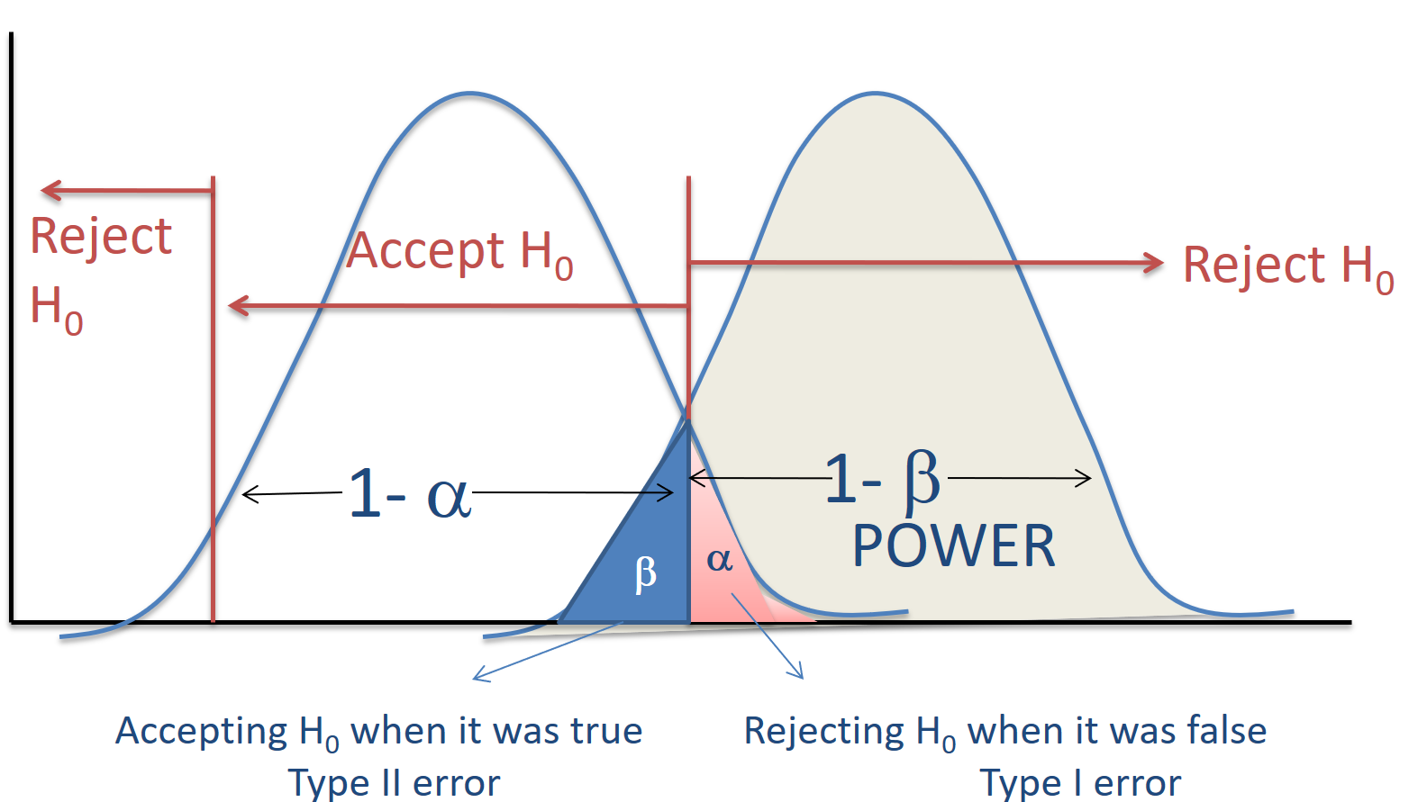
Important note: The diagram above refers to “accepting” the null hypothesis. Note that—as we have already discussed—we can not use a hypothesis test to “accept” a null hypothesis.
When should you care about power?
- Planning sample size – adequately large sample to detect expected effect
- power = .80 is common, more and more people are using .90
- Interpreting results – understand whether or not you had good chance of detecting existing effect
- particularly when results not significant
- do not assume that failure to reject null implies the null is true (see table below)
| Hypothesis Test | Power | Interpretation |
|---|---|---|
| Significant | High | Likely that \(H_0\) is false |
| Significant | Low | Likely that \(H_0\) is false; rejected null despite low power |
| Non-significant | High | Likely that \(H_0\) is true; no difference exists (or the effect is very small) |
| Non-significant | Low | Don’t know; May not have had enough power to detect effect, or effect does not actually exist |
What affects power?
- Sample size
- power increases as sample size increases
- Criterion for rejecting null (alpha, \(\alpha\))
- more power for more lenient criterion
- 5% has more power than 1%
- 1-tailed test has more power than 2-tailed test
- trade off with Type I error rate
- more power for more lenient criterion
- Effect size
- more power for larger effects
- effect size can be increased by
- increasing m1 - m2
- decreasing s
Problems with Hypothesis Testing (that are related to power and effect size)
There are two common interpretation errors with respect to hypothesis tests:
Error 1 – Assuming that failure to reject the null hypothesis implies that the null is true:
- depends on statistical power
- when statistical power is low there is little chance of getting a significant result even when the null is false
Error 2 – Assuming that a statistically significant result must be practically important:
- with large enough sample, even trivial effects will be significant
- must interpret effect size
12.1.2 Notes on Effect Size
A hypothesis test does not evaluate the size of the effect of the treatment. An effect size provides a measurement of the magnitude of the effect. Effect sizes are usually presented in standardized units.
One common effect size you will see when means are compared is Cohen’s d. Cohen’s d is the difference between means in standard deviation units:
\[d = \frac{M_1-M_2}{SD_{pooled}}\]
Above,
- \(d =\) Cohen’s d, meaning the difference between two means measured in units of the pooled standard deviation.
- \(M_1 =\) mean of group 1
- \(M_2 =\) mean of group 2
- \(SD_{pooled} =\) Pooled standard deviation of groups 1 and 2.
| Value of Cohen’s d | Evaluation of Effect Size |
|---|---|
| \(0<d<0.2\) | Small effect |
| \(0.2 < d < 0.8\) | Medium effect |
| \(d > 0.8\) | Large effect |
12.1.3 Conducting a Power Analysis
In research you conduct during or after your program at IHP, there is a good chance that you will need to conduct a power analysis in order to determine how many participants you should include in your study or determine what effect size you are able to detect with a given sample. You will need to balance the results of your power analysis with feasibility—how many participants you can actually recruit. Sometimes, those numbers will not be the same, and you’ll need to come up with a plan on how to handle that.
G*Power is a free power calculation software than can calculate the power of a wide range of study designs.
You can download and find information about G*Power here: https://www.psychologie.hhu.de/arbeitsgruppen/allgemeine-psychologie-und-arbeitspsychologie/gpower
To use G*Power, you’ll need to know the following information regarding you study design:
- The test family (t-test, F, chi-square, regression, etc.) appropriate for your design
- Estimated effect size (if you can, enter it directly, or enter M/SDs and let G*Power calculate the effect size—see the video below).
- Alpha (use .05)
- Power (calculate power .80 or .90 recommended)
- Tails (use a two-tailed test)
Relevant resources:
- In the video linked here, you can see how G*Power is used to conduct a power analysis for a dependent samples t-test: https://www.youtube.com/watch?v=nVBwhJ9gonQ
Another great feature of G*Power is that you can create tables and graphs for your analysis.
Please spend some time this week exploring G*Power. It is a very useful and widely-used tool.
12.1.4 Optional Resources
The following resources related to power and effect size may also be useful, but are not necessary to read:
Cohen, J. (1992). A power primer. Psychological Bulletin, 112(1), 155. http://www.bwgriffin.com/workshop/Sampling A Cohen tables.pdf. – This is considered a classic reading on power.
Ferguson, C. J. (2009). An effect size primer: A guide for clinicians and researchers. Professional Psychology: Research and Practice, 40(5), 532. https://www.researchgate.net/profile/Christopher_Ferguson/publication/232558476_An_Effect_Size_Primer_A_Guide_for_Clinicians_and_Researchers/links/0c960530411994b314000000.pdf.
12.2 P-Values
Over the past few decades, the controversy surrounding p-values has been building. Nevertheless, they remain a constant presence in scientific research. The quest for \(p<.05\) is reinforced by the peer-review and publishing process, as many journals will not accept/publish studies where the researcher failed to reject the null hypothesis.
After looking through the articles below, you should be able to answer the following question confidently: What is the correct interpretation of a p-value?
Please read the following article:
- Nuzzo, R. (2014). Statistical errors. Nature, 506(7487), 150. http://folk.ntnu.no/slyderse/Nuzzo%20and%20Editorial%20-%20p-values.pdf.
12.2.1 Optional Resources
The following resource related to p-values may also be useful and interesting, but is not necessary to read:
- Ioannidis, J. P. (2005). Why most published research findings are false. PLoS Medicine, 2(8), e124. https://doi.org/10.1371/journal.pmed.0020124.
12.3 Assignment
In this week’s assignment, you will practice calculating sample sizes and effect sizes, with the goal of improving your research/experimental design capabilities. It is important to make an analysis plan that includes sample/effect size analysis before you do any research! For data that is already collected, it is important for you to be able to determine the effect size that your data allows you to detect.
This assignment is a good opportunity to use your own data, if you wish. If you do want to use your own data, just replace the variables in the instructions below with variables from your own dataset.
If you want to use provided data, you should use the diabetes dataset which you can click here to download. Then run the following code to load the data into R:
if (!require(foreign)) install.packages('foreign')
library(foreign)

diabetes <- read.spss("diabetes.sav", to.data.frame = TRUE)
For the questions in this assignment, you can use G*Power, R, manual calculation, or any other tools you would like.
I personally recommend that you use G*Power for whatever you can. You can default to using a two-sided t-test model within the software.
12.3.1 Experimental Design
Task 1: Calculate Cohen’s d for the effect of gender on stabilized.glucose in the diabetes dataset. Plug the relevant numbers into the formula given below:
\[d = \frac{M_1-M_2}{SD_{pooled}}\]
The following table may also be useful:
## # A tibble: 2 x 4
##   gender count  mean    sd
## * <fct>  <int> <dbl> <dbl>
## 1 male     169  112.  63.6
## 2 female   234  103.  43.6
You can calculate the pooled SD manually using this guide. Alternatively, you can use R to calculate it:
if (!require(ANOVAreplication)) install.packages('ANOVAreplication')
library(ANOVAreplication)

data <- data.frame(y=diabetes$stabilized.glucose,g=diabetes$gender)
pooled.sd(data)
Task 2: Now calculate the same Cohen’s d using just R alone. You can run the following code:
if (!require(psych)) install.packages('psych')
library(psych)

cohen.d(diabetes,"gender")
Task 3: Now calculate the Cohen’s d for the effect of gender on total_cholesterol, by plugging into the formula again. Compare this value to what you got in the output when you ran the cohen.d() function.
Task 4: With the diabetes dataset the way it is now (meaning that the means and standard deviations of all variables are as you can calculate in the diabetes dataset), how big of an effect of gender on total_cholesterol could the data possibly detect (if it existed), with 0.8 power. What about 0.9 power?
Task 5: Let’s say we want to be able to detect half of the effect size that you found in the previous question. How much larger would we have to make our sample? Calculate the answer for 0.8 power and 0.9 power.
Task 6: In the question above, with the effect of gender on total_cholesterol, if we fail to detect an effect, does that mean that no effect exists?
Task 7: If we are trying to determine if there is a difference between the means of two groups, what is the relationship between detectable effect size and sample size, holding standard deviation constant?
12.3.2 P-Values
Task 8: What are the arguments against the focus on p-values in statistical analysis? Do you agree with them?
Task 9: What are the arguments in favor of focusing on p-values in statistical analysis? Do you agree with them?
Task 10: Why do some researchers emphasize a focus on effect sizes over p-values?
12.3.3 Follow up and submission
You have now reached the end of this week’s assignment. The tasks below will guide you through submission of the assignment and allow us to gather questions and/or feedback from you.
Task 11: Please write any questions you have for the course instructors (optional).
Task 12: Please write any feedback you have about the instructional materials (optional).
Task 13: Knit (export) your RMarkdown file into a format of your choosing.
Task 14: Please submit your assignment to the D2L assignment drop-box corresponding to this chapter and week of the course. And remember that if you have trouble getting your RMarkdown file to knit, you can submit your RMarkdown file itself. You can also submit an additional file(s) if needed.