Chapter 5 Feb 16–21: t-tests in R

This chapter has been updated for spring 2021.

This week, our goals are to…

Review t-tests.
Run t-tests in R.
Test assumptions of t-tests in R.

Announcements and reminders:

I forgot to send out a poll to check for your availability for meetings this week. Please email Nicole and Anshul to set up either a one-on-one or group meeting, if you would like. At least one group meeting has already been scheduled this week. You should have received calendar invitations from Nicole for this already.
You may have noticed on our course calendar that Oral Exam #1 is coming up soon. Each of you should please schedule an individual meeting time with Anshul and/or Nicole for us to do your Oral Exam #1. This appointment should be scheduled between February 22 and March 5 2021. In other words, you have a two-week window to do Oral Exam #1. Some more information about Oral Exam #1 is below.

How should I prepare for the oral exam? What will it test?

The exam will test your knowledge of and skills related to the quantitative methods we have learned before February 21, 2021, meaning the first five chapters of our textbook.
The exam will test your ability to conduct some but not all of these methods in R.
You can refer to any materials you would like—course book, your notes and assignments, online sources, anything else—during the exam. Therefore, I suggest that you refresh your memory about where you can find R code that you need, so that you can copy and paste it easily. You can also copy and paste from your homework assignments during the exam. Beyond that, I recommend reviewing the statistical concepts more than R code.
More weight will be given to your knowledge and interpretation of statistical concepts than your ability to write R code.

What will happen during the exam?

The exam will likely take 1 hour,⁶⁹ depending on your level of familiarity with the content.
We will ask you a few theoretical questions.
We will ask you to open a dataset in R and run a few data preparation commands in it.
We will ask you to conduct a series of visualizations and statistical tests in R and interpret the results.
We will tell you after each task/question if you were correct or not. You can re-try some tasks on the spot if you wish. Other items can be flagged for re-testing later.
If you need to have anything re-tested, we can schedule a separate time for that or we can re-test you on these items during Oral Exam #2 in a few weeks, to streamline the process for you.
We will try to be efficient during the oral exam so that we don’t run out of time.

Why do we do oral exams in this course?

Since ours is an asynchronous course in which we do not have regular class meetings, we instructors do not have an opportunity to interact with each of you to make sure that you are comfortable with all of the content and skills. If this were an in-person course with regular class meetings, we would use a flipped classroom model in which you would read this textbook before coming to class and then we would do lab-style activities during the class meeting in which you would apply skills in R and interpret results, together as a group. The Oral Exams in this course are used to replace these in-person interactions and make sure that each student has at least three hours of interaction with an instructor while answering quantitative questions during the semester.

Please e-mail both Anshul and Nicole with times when you could do your Oral Exam #1.

5.1 Independent samples t-test in R

Earlier in this course, we learned about independent samples t-tests and you conducted a t-test using an online tool. However, we did not learn how to conduct t-tests in R. Below, we use an abbreviated example that you have seen before to run an independent samples t-test in R.

When we first learned about t-tests, we used an example in which we were testing a blood pressure medication. We wanted to compare two separate groups—treatment and control—to see if their mean change in blood pressure over 30 days is the same or different.

We can load this blood pressure data into R like this:

treatment <- c(-8, -14.8, -6.8, -11.6, -10.2, -11.6, -4.8, -6.5, -9.9, -17.2, -10.7, -11.9, -8.7, -11.6, -8.6, -8.3, -10.9, -14.1, -8.8, -12.4, -14.1, -16.8, -1.8, -10.8, -15.1, -8.5, -11.2, -9.8, -10.9, -12.8, -9.2, -10.1, -12.2, -8.8, -8.5, -7.5, -10.2, -6.2, -11.4, -8.1, -15.3, -6.3, -7.2, -5.9, -13.4, -16.8, -10.7, -10.9, -12.9, -13.1)

control <- c(0, -3.5, -2.6, 3.7, -1.1, -0.6, -0.3, -1.5, 4.9, -1.8, -0.3, 0.2, -0.6, -6, -4.1, -0.5, -2.6, 0.4, 0.5, 1.9, -1, -0.1, 1.6, -3.2, -1, -3.7, 1.8, -4.2, 1, -2.2, 2, 5.5, 1.5, 1, 3.7, -1.5, -3.3, -2.7, -4.3, -7, -1.4, 5.2, 3.8, 4.6, -1.5, 2.1, -5.1, 0.5, 3.5, -0.7)

bpdata <- data.frame(group = rep(c("T", "C"), each = 50), SysBPChange = c(treatment,control))

Here is what we asked the computer to do for us above:

treatment <- c(...) – Create a column⁷⁰ of data (that is not part of any dataset⁷¹) called treatment which contains 50 numbers. The 50 numbers are given by us to the computer inside of the c(...) portion of the command. The c is how a new column of data is defined in R.
control <- c(...) – Create a column of data (that is not part of any dataset) called control which contains 50 numbers, again defined using the c(...) notation.
bpdata <- data.frame(...) – Create a new dataset (technically called a data frame in R) with two variables (columns): group and SysBPChange (which stands for systolic blood pressure change).
- group = rep(c("T", "C"), each = 50) – Create a variable in the new dataset called group which will have 100 observations (rows). Observations in the first 50 rows will have a value of T and observations in the next 50 rows will have a value of C.
- SysBPChange = c(treatment,control)) – Create a variable in the new dataset called SysBPChange which will contain the values in the already-existing column of data called treatment and then the values in the already-existing column of data called control.

It is not essential for you to fully understand the commands above or use them in the future without explicit guidance.

Now bpdata, treatment, and control should appear in your Environment tab in RStudio. You can run the following commands to inspect these three new items:

View(bpdata)
View(treatment)
View(control)

Remember: Do not leave the View(...) commands above in your RMarkdown file, because doing so may cause problems when you try to Knit (export) your work!

Using the code below that we have used before, we can examine the dataset that we just created:

if (!require(dplyr)) install.packages('dplyr')
library(dplyr)

dplyr::group_by(bpdata, group) %>% 
dplyr::summarise(
  count = n(), 
  Mean_SysBPChange = mean(SysBPChange, na.rm = TRUE),
  SD_SysBPChange = sd(SysBPChange, na.rm = TRUE)
  )

## # A tibble: 2 x 4
##   group count Mean_SysBPChange SD_SysBPChange
## * <fct> <int>            <dbl>          <dbl>
## 1 C        50            -0.38           2.95
## 2 T        50           -10.5            3.22

Above, we can see that we have successfully created the dataset bpdata in which there are 50 observations in the treatment group—identified as T—and their mean change in systolic blood pressure was -10.5 mmHg, with a standard deviation of 3.2 mmHg. And there are 50 observations in the control group—identified as C—and their mean change in systolic blood pressure was -0.4 mmHg, with a standard deviation of 2.9 mmHg.

We can also visualize our data in bpdata using a boxplot:

boxplot(SysBPChange~group,bpdata)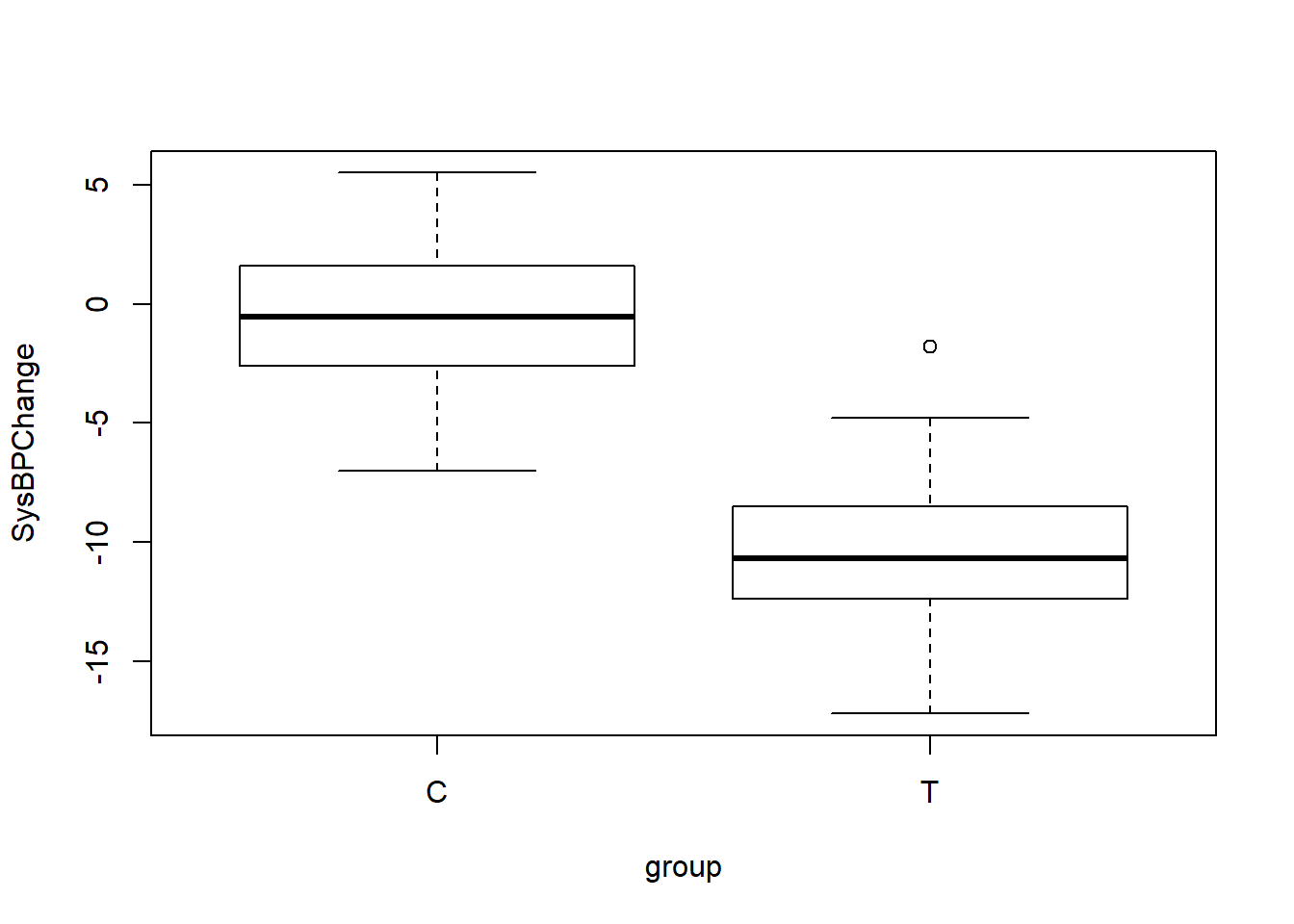

Now it is time to run our t-test in R, using the code below:

t.test(SysBPChange ~ group, data = bpdata)

## 
##  Welch Two Sample t-test
## 
## data:  SysBPChange by group
## t = 16.354, df = 97.233, p-value < 2.2e-16
## alternative hypothesis: true difference in means is not equal to 0
## 95 percent confidence interval:
##   8.872546 11.323454
## sample estimates:
## mean in group C mean in group T 
##          -0.380         -10.478

Here’s what we asked the computer to do with the code above:

t.test(...) – Run an independent samples t-test.
SysBPChange ~ group – Our outcome variable of interest—which we could also call our dependent variable—is SysBPChange. Our group identification variable—which also could be called our independent variable—is group.
data = bpdata – The dataset containing the variables used for this t-test is called bpdata.

And now we can interpret the results of the t-test from the output we received, pending the diagnostic tests later in this section:

The 95% confidence interval of the effect size in the population is 8.9–11.3 mmHg. This means that there is a 95% chance that in the entire population (not our sample of 100 subjects), people who take the medication improve (decrease) their systolic blood pressure by at least 8.9 mmHg and at most 11.3 mmHg on average, relative to those who don’t take the medication.
The p-value is extremely small, lower than 0.001.⁷²
We have sufficient evidence—pending the diagnostic tests later in this section—to reject the null hypothesis and conclude that in the population, the systolic blood pressures of those who take the medication reduce more than the systolic blood pressures of those who do not take the medication, on average.

Before we can consider the results of the t-test above to be trustworthy, we must first make sure that our data passes a few diagnostic tests of assumptions that must be met. These assumptions are discussed later in this chapter.

5.2 Paired sample t-test

A paired sample t-test compares an outcome of interest that is measured twice on the same set of observations. Another name for a paired sample t-test is a dependent sample t-test (as a counterpart to the independent samples t-test we learned earlier). More specifically, the paired sample t-test compares the means of an outcome of interest that is measured twice within a single sample.

We will use an example to practice using a paired samples t-test. Imagine a situation in which 50 students are sampled from a larger population of students. These students are learning a particular skill. They are first pre-tested on their initial ability to perform the skill, then they participate in an educational intervention to improve their abilities to do the skill, and finally they take a post-test at the end of the procedure. We want to know if students in the larger population of students are able to perform the skill better after they participate in the educational intervention than before.⁷³ Since the two means—pre-test and post-test scores—we want to compare come from the same observations (students), a paired sample t-test is the correct inference procedure to use.

The research design is diagrammed in the chart below:

Now that we have identified a question to answer, let’s load our data into R using the following code.

post <- c(82.7, 71.7, 66.9, 67.9, 87.3, 65.5, 72.2, 81.2, 65.2, 79.1, 80.9, 94.6, 83.7, 76.8, 78.5, 70.4, 61.4, 93.3, 70.8, 71.7, 77.4, 70.8, 65.7, 69.6, 72.4, 73.3, 81.8, 71.6, 73.6, 72.8, 84.5, 73.3, 67.1, 80.7, 82.5, 84.1, 86.1, 84.7, 73.8, 74.5, 70.7, 80.5, 80.6, 61.2, 81.1, 78.6, 67.3, 67.6, 77.2, 66.8)

pre <- c(55.4, 82.8, 88.1, 74.4, 64.9, 73.9, 90.6, 90.6, 86.8, 83.5, 85.4, 87.3, 69.1, 84.4, 69.4, 38.5, 64, 67.5, 68, 86.8, 81.5, 56.6, 51.9, 65.5, 82.4, 65.3, 81.8, 58.9, 60.9, 66.1, 72.7, 45.5, 69.6, 70.1, 79.7, 68.4, 75.7, 39.3, 75, 63.9, 76.7, 67.2, 71.6, 62.9, 76.5, 90.1, 66.8, 71.8, 77, 65.2)

tests <- data.frame(pre,post)

Above, we created a dataset called tests which contains 50 observations (students, in this case). The dataset tests contains the variable pre, which holds all of the pre-test scores; and tests contains the variable post, which holds all of the post-test scores.

We can use familiar commands to describe our data:

summary(tests$pre)

##    Min. 1st Qu.  Median    Mean 3rd Qu.    Max. 
##   38.50   65.22   70.85   71.36   81.72   90.60

sd(tests$pre)

## [1] 12.47582

summary(tests$post)

##    Min. 1st Qu.  Median    Mean 3rd Qu.    Max. 
##   61.20   70.47   73.70   75.47   81.05   94.60

sd(tests$post)

## [1] 7.721632

We can visualize the pre and post-test scores using a boxplot:

boxplot(tests$pre,tests$post)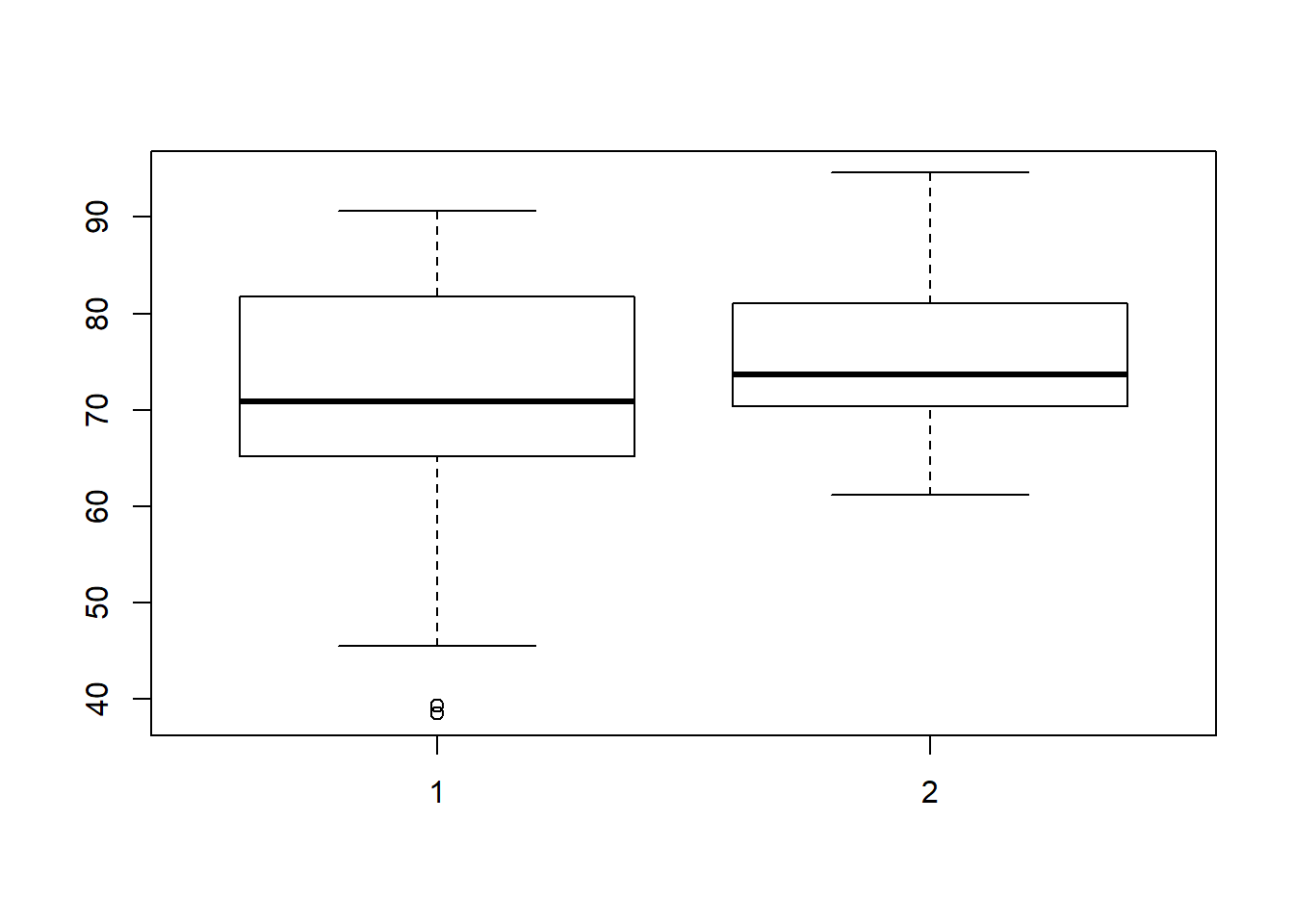

We can now write hypotheses for the paired sample t-test that we will use:

$H_0\text{: } \mu_{pre} = \mu_{post}$. The null hypothesis is that in the population of students from which the sample of 50 students were selected, students’ pre-test and post-test scores are the same on average.
$H_A\text{: } \mu_{pre} \ne \mu_{post}$. The alternate hypothesis is that in the population of students from which the sample of 50 students were selected, students’ pre-test and post-test scores are not the same on average.

As with the independent samples t-test, our hypotheses relate to the population from which our sample was selected, rather than our sample itself. Our goal is to find out if the educational intervention is associated with an improvement in test score in the entire population of students, not only in our sample of 50 students. We already know that in our sample of 50 students, the average pre-test score is 71.4 test points and the average post-test score is 75.5 test points; so the average difference is 4.1 test points. But what is this difference in our population? That’s what the paired sample t-test will help us figure out, below.

We can run the following code to run our paired sample t-test on our student data:

t.test(tests$post,tests$pre, paired=TRUE)

## 
##  Paired t-test
## 
## data:  tests$post and tests$pre
## t = 2.1061, df = 49, p-value = 0.04034
## alternative hypothesis: true difference in means is not equal to 0
## 95 percent confidence interval:
##  0.1885839 8.0394161
## sample estimates:
## mean of the differences 
##                   4.114

Here’s what we asked the computer to do with the code above:

t.test(...) – We want to do a t-test.
tests$post – One variable we want to include in the t-test is the variable post within the dataset tests.
tests$pre – Another variable we want to include in the t-test is the variable pre within the dataset tests.
paired=TRUE – This is going to be a paired t-test, meaning that each value of pre corresponds to a value of post. The samples are not independently taken from different groups of people.

We learn the following from the output of our paired sample t-test, pending the diagnostic tests later in this section:

The 95% confidence interval is 0.2–8.0 test points. This means that on average in our entire population of students (not the 50 students in our study), we are 95% certain that students who participate in this educational intervention will improve their score by at least 0.2 test points and no more than 8.0 test points from the pre-test to the post-test.
The p-value is 0.04. This means that we are 96% certain that the alternate hypothesis is true. It also means that if we reject the null hypothesis, there is a 4% chance that this would be an error.
This is an example of a situation in which the discretion of the researcher is very important. On one hand, our 95% confidence interval is entirely above 0. On the other hand, an effect size of just 0.2 test points —which is within the range of possibilities since it is within the 95% confidence interval—is not a very meaningful average improvement from pre to post-test. In such a situation, it is important to communicate transparently about your results. You can report the exact 95% confidence interval and p-value and then explain that 0.2 test points is not a very meaningful effect size, but 8.0 is. You can say that there is limited but not definitive evidence to support your alternate hypothesis. This is an example of a responsible approach to running and reporting your analysis.

5.3 T-test diagnostic tests of assumptions

Most statistical tests that are used for inference require that a unique set of assumptions about the data being used are met. The t-tests that we have learned about in this chapter are no exception to this. Before we can trust the results of any t-test that we conduct, we must run a series of diagnostic tests to check if our data meet all necessary assumptions.

For an independent samples t-test, the data must satisfy the following three conditions for the t-test results to be trustworthy: independence of observations, samples must be approximately normally distributed, and samples must have approximately the same variances. For a paired sample t-test, these assumptions are modified, as you will read below.

Below, you will find a guide to conducting diagnostic tests to test all three assumptions of t-tests. If the two samples you are using for your t-test both satisfy the necessary assumptions below, then you know that you can trust the results of your t-test.

5.3.1 Independence of observations

This assumption is not one that you will test in R. Instead, assuring the independence of observations is a practical and theoretical question that you need to answer for yourself based on your data. Furthermore, the independence assumption is not required in the same way for a paired sample t-test. It is only required for an independent sample t-test.

The independence assumption requires that each individual data point that is included in one or more samples in the t-test comes from a separate observation. For example, in our blood pressure scenario from earlier in this chapter, no two blood pressure measurements should come from the same person. Each blood pressure measurement should come from a different person.

Furthermore, the independence assumption requires that the outcome of interest (that is measured to include in the samples in the t-test) are not correlated with each other in any way. This means that one observation’s value of the dependent variable should not influence another observation’s value of the dependent variable. In the context of our blood pressure example, this means that one person’s blood pressure—or adherence to the medication regime, which in turn could influence blood pressure—should not influence another person’s blood pressure. All participants should be separate from each other and not have an influence on one another.

For a paired sample t-test, the two samples will of course not be independent of one another. For example, a student’s pre-test score and their post-test score will be influenced by each other. However, the observations in a paired sample t-test should be independent of each other. This means that the students in our example earlier in this chapter should not influence each other’s pre and post-test scores.

When you run a t-test, you should take a moment to double-check if the way in which your data was collected and measured meets the requirements of this independence assumption or not.

5.3.2 Samples normally distributed

This assumption requires that the data in both samples used in the t-test are approximately normally distributed. More specifically, the assumption requires that the outcome being measured is normally distributed in the population, although we typically just test this by testing the normality of the samples. This assumption is required for both independent samples and paired sample t-tests.

Here are some examples from the data we used earlier in this chapter:

In our blood pressure scenario, the treatment group and control group blood pressure change measures must be normally distributed.
In our student skills pre and post-test example, the pre-test scores and the post-test scores must be normally distributed.

There are a number of ways to test normality. Multiple methods are demonstrated below. I recommend that you try all of these methods when attempting to determine if a distribution of data is normally distributed or not, just to be on the safe side. Before we begin testing for normality, let’s re-load some of our data from earlier which we will use for the demonstration.

You can re-run the code below to load the student pre and post-test data that we used earlier in the chapter:

post <- c(82.7, 71.7, 66.9, 67.9, 87.3, 65.5, 72.2, 81.2, 65.2, 79.1, 80.9, 94.6, 83.7, 76.8, 78.5, 70.4, 61.4, 93.3, 70.8, 71.7, 77.4, 70.8, 65.7, 69.6, 72.4, 73.3, 81.8, 71.6, 73.6, 72.8, 84.5, 73.3, 67.1, 80.7, 82.5, 84.1, 86.1, 84.7, 73.8, 74.5, 70.7, 80.5, 80.6, 61.2, 81.1, 78.6, 67.3, 67.6, 77.2, 66.8)

pre <- c(55.4, 82.8, 88.1, 74.4, 64.9, 73.9, 90.6, 90.6, 86.8, 83.5, 85.4, 87.3, 69.1, 84.4, 69.4, 38.5, 64, 67.5, 68, 86.8, 81.5, 56.6, 51.9, 65.5, 82.4, 65.3, 81.8, 58.9, 60.9, 66.1, 72.7, 45.5, 69.6, 70.1, 79.7, 68.4, 75.7, 39.3, 75, 63.9, 76.7, 67.2, 71.6, 62.9, 76.5, 90.1, 66.8, 71.8, 77, 65.2)

tests <- data.frame(pre,post)

Now that we have loaded our data, we are ready to test normality. For the examples below, we will only test normality on the pre-test data. Keep in mind that you would also have do all of these tests on the post-test data as well. In other words: make sure you test normality in both samples that you are using the t-test to compare, not just one.

The first method we will use to test normality is visual inspection. One of the fastest was to do this is simply to make a histogram, which you are already familiar with.

Histogram of pre-test data:⁷⁴

hist(tests$pre)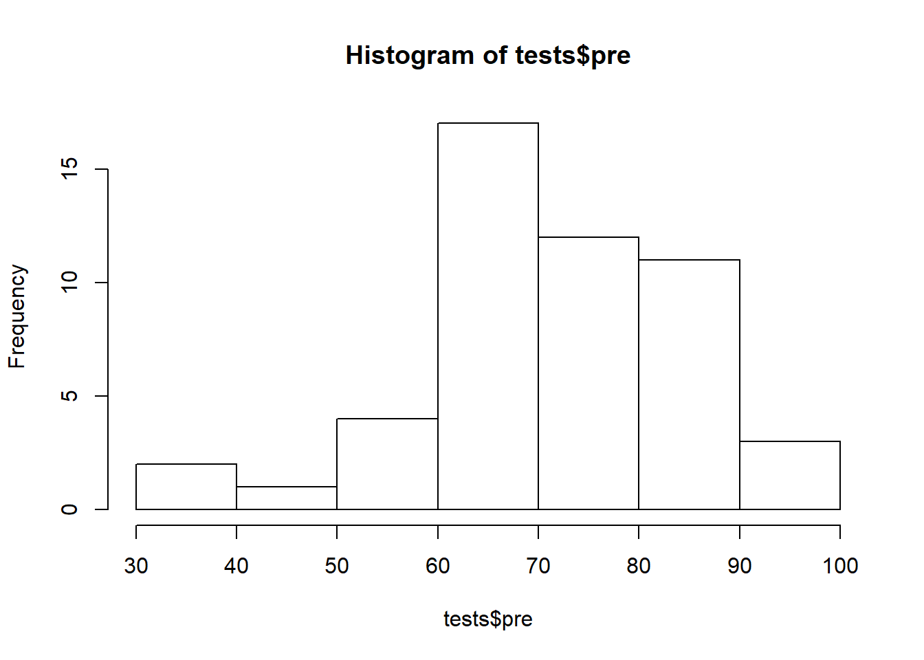

Above, the pre-test data looks like it might be normal but it isn’t very clear. The histogram makes it look like there are more observations above the mean than below the mean. Let’s continue checking for normality in different ways to see if we can get a more definitive answer.

The next method is to make what is called a quantile-quantile normal plot, or QQ plot for short.

Run the code below to make this plot:⁷⁵

if (!require(car)) install.packages('car')
library(car)

qqPlot(tests$pre)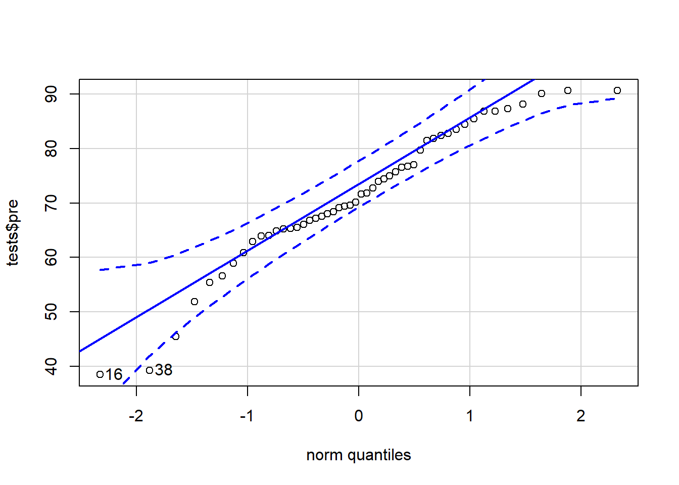

## [1] 16 38

In the code above, we gave our variable of interest—tests$pre—into the qqPlot(...) function from the car package. It then produced a QQ plot for us. A QQ plot plots our data on the y-axis against theoretical normal distribution quantiles on the x-axis. It is not required for you to fully understand the process by which the graph is created. It is most important for you to know how to interpret the graph.

If your data is perfectly normally distributed, your data points will all fall along the solid blue line. Of course, some deviation from this line is acceptable. Confidence bands have been drawn in dotted blue lines. If your data falls within these bands, there is a high chance that they were drawn from a normal distribution. If any data points fall outside of these bands, you might want to consider either removing those observations from your analysis or trying a test other than a t-test.

Now that we have covered two visual ways to inspect your data for normality, there is a third way that is non-visual and uses a hypothesis test to check for normality. This is called the Shapiro-Wilk normality test.

These are the hypotheses for the Shapiro-Wilk normality test:

$H_0$: The data are normally distributed.
$H_A$: The data are not normally distributed.

And here is the code to run the test:

shapiro.test(tests$pre)

## 
##  Shapiro-Wilk normality test
## 
## data:  tests$pre
## W = 0.95465, p-value = 0.05311

Above, we gave the tests$pre variable to the shapiro.test(...) function and it ran the test on our data.

We interpret this test using the p-value, which in this case is just above 0.05. This means that there is approximately 95% support for the alternate hypothesis, which in this case is that the data is not normally distributed. This evidence is strong enough to at least suggest that our data might not be normal. Therefore, in this case, our data might violate the normality assumption of the t-test. Therefore, we should not use a t-test on this data and we should not trust the results given by any t-tests which used this data.

If the p-value had been higher and the visual inspection methods had also made the data look more normal, then we would have been fine. But as it stands right now, we might not be. One solution could be to remove a few outliers and re-run our t-test. And another could simply be to use a different type of test to answer our question.

5.3.3 Homogeneity of variances

The third assumption that must be satisfied is that the variance of the two samples being compared in the t-test should have approximately the same variance as each other. This is required for only the independent samples t-test, not the paired sample t-test.

Let’s reload our data from our independent t-test that we ran earlier in this chapter, which tested the hypothesis about blood pressure medication.

This code loads the data:

treatment <- c(-8, -14.8, -6.8, -11.6, -10.2, -11.6, -4.8, -6.5, -9.9, -17.2, -10.7, -11.9, -8.7, -11.6, -8.6, -8.3, -10.9, -14.1, -8.8, -12.4, -14.1, -16.8, -1.8, -10.8, -15.1, -8.5, -11.2, -9.8, -10.9, -12.8, -9.2, -10.1, -12.2, -8.8, -8.5, -7.5, -10.2, -6.2, -11.4, -8.1, -15.3, -6.3, -7.2, -5.9, -13.4, -16.8, -10.7, -10.9, -12.9, -13.1)

control <- c(0, -3.5, -2.6, 3.7, -1.1, -0.6, -0.3, -1.5, 4.9, -1.8, -0.3, 0.2, -0.6, -6, -4.1, -0.5, -2.6, 0.4, 0.5, 1.9, -1, -0.1, 1.6, -3.2, -1, -3.7, 1.8, -4.2, 1, -2.2, 2, 5.5, 1.5, 1, 3.7, -1.5, -3.3, -2.7, -4.3, -7, -1.4, 5.2, 3.8, 4.6, -1.5, 2.1, -5.1, 0.5, 3.5, -0.7)

bpdata <- data.frame(group = rep(c("T", "C"), each = 50), SysBPChange = c(treatment,control))

Now that we have the bpdata dataset loaded once again, we can test to see if the treatment and control groups in this data have homogenous variances (meaning similar variances as each other).

We will ask R to run a hypothesis test for us to test for homogeneity of variances. These are the hypotheses for this test:

$H_0$: The two samples of data do have similar variances.
$H_A$: The two samples of data do not have similar variances.

To conduct this hypothesis test, we will use the following code:

var.test(SysBPChange ~ group, data = bpdata)

## 
##  F test to compare two variances
## 
## data:  SysBPChange by group
## F = 0.83685, num df = 49, denom df = 49, p-value = 0.5354
## alternative hypothesis: true ratio of variances is not equal to 1
## 95 percent confidence interval:
##  0.4748926 1.4746881
## sample estimates:
## ratio of variances 
##          0.8368504

Here’s what the code above asked the computer to do:

var.test(...) – Run the var.test(...) function, which runs what is called an F-test for homogeneity of variances.
SysBPChange ~ group – The data we want to check for homogeneity of variances is in the dependent variable SysBPChange and this data is divided up into two groups according to the group variable.
data = bpdata – The variables used in this test come from the dataset called bpdata.

We will evaluate the results of this hypothesis test by looking at the p-value, which in this case is approximately 0.54. This is a very high p-value, allowing us to easily fail to reject the null hypothesis. This means that we did not find evidence that our two samples for our t-test violate the homogeneity of variances assumption.

If this p-value had been closer to or lower than 0.05, then we would be concerned and we would have to consider using a different test to analyze our data.

5.3.4 Summary of assumptions for independent and paired t-tests

Here is a summary of which assumptions need to be tested using diagnostic tests for each type of t-test.⁷⁶

Independent samples t-test

Independence of observations⁷⁷
Normality of samples (and underlying populations; each of your two samples on their own need to be normally distributed, so you will run normality tests separately for each sample)
Homogeneity of variances (equal variances)

Paired sample t-test

Independence of observations (partially)
Normality of samples (and underlying populations)

5.3.5 When assumptions are not met

You may have noticed that in the paragraphs above, when our data violates or comes close to violating one of the t-test assumptions, you are told that you might want to use a different type of test. But what type of test would you use instead of a t-test? Here are some—though certainly not close to all—possibilities:

Wilcoxon Signed Rank test. This is used in similar situations as when a t-test is used, but the assumptions are less restrictive. If you have data that is well suited for a t-test but violates one or more t-test assumptions, the Wilcoxon Signed Rank test could be a simple solution. Run the command ?wilcox.test in R to learn more about this test. The implementation and interpretation of this test is fairly similar to those of a t-test. Both independent and paired varieties of this test are available.
Linear regression. We will learn about linear regression soon in this textbook. Linear regression is one of the most versatile and commonly used quantitative analysis methods and is often useful in situations where a t-test might otherwise be used.
Multilevel linear regression model (linear fixed effects or random effects model). We will learn about these types of models later in this textbook. These are types of linear regression models that are specifically designed to correct for situations in which standard test assumptions have been violated.

5.4 Assignment

In this week’s assignment, you will practice running a paired sample t-test. Imagine that we, some researchers, are trying to answer the following research question: Is daily weightlifting exercise associated with a change in ability to lift weight?

To answer this question, we created a study with 100 subjects. On the first day, we measured how many squats each participant could do in one minute while wearing a ten pound vest (called pre data). We then had each participant participate in an exercise program for a month. At the end of that month, we again measured how many squats each participant could do in one minute while wearing a ten pound vest (called post data).

Use the code below to load this data into R:

pre <- c(6.9, 4.8, 16.4, 19.8, 16.2, 21.1, 15, 14.9, 9.4, 16.5, 21.6, 19.3, 7.1, 31.7, 24.7, 9.8, 19.1, 3.3, 15.4, 17.9, 18.2, 19, 6.4, 3.7, 24.5, 15.9, 9.6, 29.9, 18.2, 30.6, 22.4, 21.7, 6.5, 1.4, 28.9, 13.9, 7.6, 12.9, 17, 35.8, 23.1, 14.9, 18.3, -0.1, 7.4, 10.6, 21.7, 4.1, 9.1, -1.9, 32, 3.9, 30.3, 23.5, 23.6, 21, 9, 29.6, 12, 15.6, 11.4, 11.3, 35.4, 20.1, 10.1, 15.2, 6.3, 14.3, 29.2, 15.5, 8.3, -8.2, 4.5, 11.7, 14.1, -1.2, 23.9, 10.7, 23.8, 17.2, 25.6, 8.4, 12.7, 15, 15.8, 34.4, 30, 19.6, 23, 13.2, 1, 31.7, 18.9, -1.5, 30.2, 8.8, 27.2, 22.5, 27, 8.8)

post <- c(18.3, 13.4, 5.1, 8.4, 8.6, 26.2, 26.2, 21, 14, 9.1, 21.7, 9.5, 25.9, 26.7, 8.9, 9.4, 14.9, 13.6, 29.2, 10.4, 13.3, 18.4, 8, 8.2, 5.3, 27.7, 18.9, -0.9, 22, 11.5, 4.3, 26.9, 30, 13.6, 22, 15.4, 8.7, 11.7, 33, 31.3, 21.6, 25.7, 15.3, 17, 10, 32.8, 26.4, 19.4, 15.3, 25.4, 22.6, 10, 17.4, 27.9, 26, 24.7, 16.1, 21.3, 22, 5.6, 14.7, 23, 23.3, 31.1, 21.3, 24.5, 12.6, 13.9, 18.7, 18.5, 10, 17.5, 20.6, 22, 19.4, 14.3, 15.5, 12, 19.4, 15, 22.8, 9.2, 22.4, 22.9, 16.3, 23.2, 28.8, 15.3, 18, 13.6, 25.8, 28.7, 19.7, 17.5, 14.8, 9.5, 16, 29.1, 11.1, 18.2)

exercise <- data.frame(pre,post)

You now have a dataset called exercise that you will use for this assignment. exercise contains two variables: pre and post.

This week, instead of asking you to follow particular steps, now you will choose which steps you need to follow to responsibly conduct a complete analysis to answer this research question about exercise. You can use the content in this chapter and your own previous work on t-tests to guide you. Please provide all descriptive statistics, inferential tests, interpretations, and diagnostic tests necessary to answer the research question. You can ask instructors and each other for help along the way.

Use an RMarkdown file to do this assignment. Once you are done, Knit the RMarkdown file into a format of your choosing and submit the knitted file to D2L.

Please also remember to email Anshul and Nicole with one or more times at which you can do your Oral Exam #1 between February 22 and March 5 2021.

But it could take less than an hour and it could take more than an hour. Both have happened before and are perfectly fine. The goal is not to be fast. The goal is to do everything at a high quality level.↩︎
This is technically called a vector in R.↩︎
This is technically called a data frame in R↩︎
The test output reports: p-value < 2.2e-16. 2.2e-16 means $2.2*10^{-16} = 0.00000000000000022$, which is a very small number! This is telling us that there is an extremely small chance that rejecting the null hypothesis would be a mistake.↩︎
This is a variety of within-subjects research design.↩︎
This code could also just be hist(pre) since pre also exists in our data on its own as a column of data that is not inside of a dataset. To make a histogram of treatment and control groups from our blood pressure example, you can run hist(treatment) and hist(control), without using the dataset bpdata as part of the command, since treatment and control are also loaded on your computer as separate columns of data that are not associated with a dataset.↩︎
This code could also just be qqPlot(pre) since pre also exists in our data on its own as a column of data that is not inside of a dataset. To make a histogram of treatment and control groups from our blood pressure example, you can run qqPlot(treatment) and qqPlot(control), without using the dataset bpdata as part of the command, since treatment and control are also loaded on your computer as separate columns of data that are not associated with a dataset.↩︎
This section was added on January 19 2021.↩︎
This list item accidentally mentioned normality when this chapter was initially published. The mistake was corrected in early March 2021.↩︎