Chapter 25 More than two samples from normal distributions
Motivating scenarios: We are interested to investigate the difference between the means of more than two samples.
Learning goals: By the end of this chapter you should be able to
- Explain the multiple testing problem.
- Explain how ANOVA attempts to solve the multiple testing problem.
- Visually identify and mathematically interpret various “sums of squares”.
- Calculate an F statistic and relate this to the sampling distribution.
- Conduct appropriate “post-hoc” tests.
25.1 Setup
We often have more than two groups. For example - we might want to know, not just if a fertilizer is better than a control, but which of a number of fertilizers have different impacts on plant growth.
Or for the extended example in this chapter, if ambient temperature can influence body temperature in rodents, like the round-tailed ground squirrel, Spermophilus tereticaudus. In this experiment, Wooden and Walsberg (2004) put squirrels in environments that where 10°C (cold), 35°C (warm), and 45°C (hot), and measured their body temperature. The data are plotted in
#first lets load the data
sqrl <- read_csv("https://raw.githubusercontent.com/ybrandvain/biostat/master/data/sqrl.csv")
# now lets order data from coldest to warmest for a pretty plot
sqrl <- mutate(sqrl, ambient_temp = fct_relevel(ambient_temp, "cold", "warm", "hot"))

ggplot(sqrl, aes(x = ambient_temp, y = body_temp, color  = ambient_temp))+
  geom_jitter(height = 0, width = .2, size = 2, alpha = .35, show.legend = FALSE)+
  stat_summary(fun.data = "mean_cl_normal", geom = "errorbar", width = .2, color = "black")+
  scale_color_manual(values = c("blue", "orange", "red"))

  include_graphics("https://upload.wikimedia.org/wikipedia/commons/thumb/1/19/Spermophilus_tereticaudus_01.jpg/256px-Spermophilus_tereticaudus_01.jpg")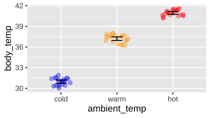

25.1.1 Review: Linear models
We can, and will, think about this like a linear model.
sqrl_lm <- lm( body_temp ~ ambient_temp, data = sqrl)
sqrl_lm
##
## Call:
## lm(formula = body_temp ~ ambient_temp, data = sqrl)
##
## Coefficients:
## (Intercept) ambient_tempwarm ambient_temphot
## 30.960 6.254 10.000We can write down the linear equation as follows:
\[\begin{equation} \begin{split}\text{body temp}_i = 30.960 + 6.254 \times WARM + 10 \times hot \end{split} \tag{25.1} \end{equation}\]
And we can find the predicted body temperature for each ambient temperature as follows:
\[\begin{equation} \begin{split} \hat{Y}_\text{Cold ambient} &= 30.960 + 6.254 \times WARM + 10 \times HOT. \\ &= 30.960 + 6.254 \times 0 + 10 \times 0 . \\ &= 30.960 \\ \\ \hat{Y}_\text{Warm ambient} &= 30.960 + 6.254 \times WARM + 10 \times HOT. \\ &= 30.960 + 6.254 \times 1 + 10 \times 0 . \\ &= 30.960 + 6.254 \\ & =37.214\\ \\ \hat{Y}_\text{Hot ambient} &= 30.960 + 6.254 \times WARM + 10 \times HOT. \\ &= 30.960 + 6.254 \times 0 + 10 \times 1 . \\ &= 30.960 + 10 \\ & =40.960 \\ \end{split} \tag{25.2} \end{equation}\]
So that’s all good, and equals the means, as we would like
sqrl %>%
  group_by(ambient_temp) %>%
summarise(mean_body_temp = mean(body_temp)) %>% kable(digits = 4)| ambient_temp | mean_body_temp |
|---|---|
| cold | 30.9600 |
| warm | 37.2143 |
| hot | 40.9600 |
But the t-values and p-values are weird
tidy(sqrl_lm) %>% kable(digits = 4)| term | estimate | std.error | statistic | p.value |
|---|---|---|---|---|
| (Intercept) | 30.9600 | 0.1157 | 267.4733 | 0 |
| ambient_tempwarm | 6.2543 | 0.1617 | 38.6701 | 0 |
| ambient_temphot | 10.0000 | 0.1637 | 61.0892 | 0 |
Specifically, we have three pairs of p and t values.
- t and p values associated with
(Intercept)(\(t = 267\), \(2.32 \times 10^{-91}\)), describe the nonsense null hypothesis that mean temperature in cold is 0°C. - t and p values associated with
ambient_tempwarm(\(t = 39.7\), \(4.16 \times 10^{-43}\)), describe the null hypothesis that would be useful to evaluate – that mean body temperature does not differ in cold vs. warm environments.
- t and p values associated with
ambient_temphot(\(t = 61.1\), \(2.40 \times 10^{-54}\)), describe the null hypothesis that would be useful to evaluate – that mean body temperature does not differ in warm vs. hot environments.
What’s wrong with the p-values above?
- We have not compared body temperatures at warm vs hot ambient temperatures.
- We have conducted “multiple tests” on the same data set. That is because we have two p-values we’re looking at, the probability that we incorrectly reject at least one true null is no longer \(\alpha\), but is the probability of not rejecting any null hypotheses \(1-(1 -\alpha)^\text{n tests}\). So with the two interesting null hypotheses to test, with a traditional \(\alpha = 0.05\) the probability of not reject any true null hypotheses is \(1-(1 -.05)^2 = 0.0975\). This is way bigger than the \(\alpha\) of \(0.05\) we claim to have.
25.1.2 Why not all paiwise t-tests?
We could solve the first issue by conducting three two-sample t-tests. But this exacerbates the second issue – now our probability of at least one false negative is \(1-(1-0.05)^3 = .143\).
bind_rows(
  t.test(body_temp ~ ambient_temp , filter(sqrl, ambient_temp != "hot"), var.equal  = TRUE) %>%
       tidy() %>% mutate(comp = "cold v warm") %>% dplyr::select(comp, p.value, t = statistic),
    t.test(body_temp ~ ambient_temp , filter(sqrl, ambient_temp != "warm"), var.equal  = TRUE) %>%
       tidy() %>% mutate(comp = "cold v hot") %>% dplyr::select(comp, p.value, t = statistic),
    t.test(body_temp ~ ambient_temp , filter(sqrl, ambient_temp != "cold"), var.equal  = TRUE) %>%
tidy() %>% mutate(comp = "warm v hot") %>% dplyr::select(comp, p.value, t = statistic)) %>% mutate(p.value = paste(round(p.value * 10^c(31,41,24),digits = 2),c("x10^-31","x10^-41","x10^-24"), sep=""))%>% kable(digits = 4)| comp | p.value | t |
|---|---|---|
| cold v warm | 1.49x10^-31 | -36.0365 |
| cold v hot | 8.77x10^-41 | -65.8778 |
| warm v hot | 1.6x10^-24 | -23.3353 |
25.1.3 More on multiple testing
. rollover test: '*So, uh, we did the green study again and got no link. It was probably a-- RESEARCH CONFLICTED ON GREEN JELLY BEAN/ACNE LINK; MORE STUDY RECOMMENDED!*'](https://imgs.xkcd.com/comics/significant.png)
Figure 25.1: The multiple testing problem according to xkcd. rollover test: ‘So, uh, we did the green study again and got no link. It was probably a– RESEARCH CONFLICTED ON GREEN JELLY BEAN/ACNE LINK; MORE STUDY RECOMMENDED!’
This classic xkcd comic provides a great cartoon of the multiple testing problem, as well as the problem of science hype and communication. If we repeatedly test true null hypotheses we’re bound to reject some by chance.
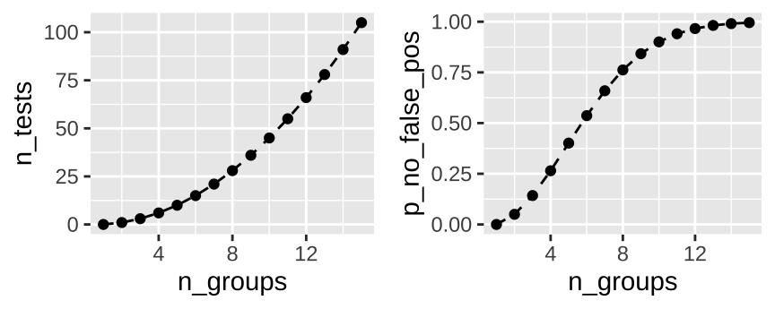
This is a potential problem when looking at differences between groups, as the number of pairwise test rapidly expand with the number of groups. How rapidly, you ask? Let’s revisit the binomial equation, where \(k\) is 2 (because we make pairs of two) and we have \(n\) groups.
\[\begin{equation} \begin{split} \binom{n}{2} &= \frac{n!}{(n-k)! \times 2!} \\ &= \frac{n\times (n-1) \times (n-2)!}{(n-2)\times 2!} \\ &= \frac{n\times (n-1) }{2} \end{split} \tag{25.3} \end{equation}\]
So, with \(n\) groups we have \(n(n-1)/2\) pairwise comparisons, and a probability of rejecting at least one true null of \(1-(1-0.05)^{n(n-1)/2}\). So all pairwise tests with fifteen groups is 105 tests, and we’re basically assured at least one will be a false positive.
25.2 The ANOVA’s solution to the multiple testing problem
Instead of testing each combination of groups, the ANOVA poses a different null hypothesis. The ANOVA tests the null hypothesis that all samples come from the same statistical population.
ANOVA hypotheses
- \(H_0\): All samples come from the same (statistical) population. Practically, this says that all groups have the same mean.
- \(H_A\): Not all samples come from the same (statistical) population. Practically this says that not all groups have the same mean.
The ANOVA makes this null by some algebraic rearrangement of the sampling distribution. That is, the ANOVA tests the null hypothesis that all groups come from the same (statistical) population based on the expected variance of estimates from the sampling distribution!!
25.2.1 Mathemagic of the ANOVA
Recall that the standard error of the mean (\(\sigma_{\overline{Y}}\)) of a sample of size \(n\) from a normal sampling distribution is the standard deviation divided by the square root of the sample size: \(\sigma_{\overline{Y}} = \frac{\sigma}{\sqrt{n}}\).

With some algebra (squaring both sides and multiplying both side by n), we see that the sample size times the variance among groups \(n \times \sigma_{\overline{Y}}^2\) equals the variance within groups \(\sigma^2\) (Equation (25.4)).
\[\begin{equation} \begin{split} \sigma_{\overline{Y}} = \sigma / \sqrt{n} \\ \sigma_{\overline{Y}}^2 = \sigma^2 / n \\ n \times \sigma_{\overline{Y}}^2 = \sigma^2 \end{split} \tag{25.4} \end{equation}\]
So, if all groups come from the same population (i.e. under the null hypothesis), \(n \times \sigma_{\overline{Y}}^2\) will equal the variance within groups \(\sigma^2\).
If all groups do not come from the same population (i.e. under the alternative hypothesis), \(n \times \sigma_{\overline{Y}}^2\) will exceed the variance within groups \(\sigma^2\).
25.2.2 Parameters and estimates in an ANOVA
So we can turn these ideas into parameters to estimate.
| Source | Parameter | Estimate | Notation |
|---|---|---|---|
| Among Groups | \(n \times \sigma_Y^2\) | Mean squares model | \(MS_{model}\) |
| Within Groups | \(\sigma^2_Y\) | Mean squares error | \(MS_{error}\) |
| Total | \(n \times \sigma_Y^2 + \sigma^2_Y\) | Mean squares total | \(MS_{total}\) |
So with this new math and algebra we can restate our null and alternative hypotheses for an ANOVA
\(H_0\): Mean squares model is not greater than mean squares error (i.e. among group variance equals zero).
\(H_A\): Mean squares model is greater than mean squares error (i.e. among group variance is not zero).
25.3 Concepts and calculations for an ANOVA
25.3.1 ANOVA partitions variance
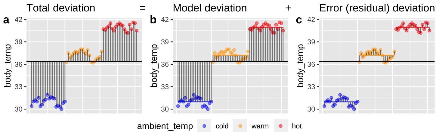
Figure 25.2: Partitioning deviations in an ANOVA. A Shows the difference between each observation, \(Y_i\), and the grand mean, \(\overline{\overline{Y}}\). This is the basis for calculating \(MS_{total}\). B Shows the difference between each predicted value \(\widehat{Y_i}\) and the grand mean, \(\overline{\overline{Y}}\). This is the basis for calculating \(MS_{model}\). C Shows the difference between each observation, \(Y_i\), and its predicted value \(\widehat{Y_i}\). This is the basis for calculating \(MS_{error}\).
Figure 25.2, really helps me understand what we are doing in ANOVA – we think about all variability in our data (a) as the sum of the variability among (b), and within groups. To do so, we first square the length of each line in Figure 25.2, and add them up. These are called the sums of squares.
sums_of_squares <- augment(sqrl_lm) %>%
  mutate(grand_mean  = mean(body_temp)) %>%
  summarise(n_groups = n_distinct(ambient_temp) ,
            n        = n(),
            ss_total = sum((body_temp - grand_mean)^2),
            ss_model = sum((.fitted   - grand_mean)^2),
            ss_error = sum((body_temp - .fitted)^2)) # or we could have just had sum(.resid^2)

sums_of_squares %>% kable(digits = 2)| n_groups | n | ss_total | ss_model | ss_error |
|---|---|---|---|---|
| 3 | 61 | 1037.21 | 1021.66 | 15.54 |
Or in math
- Sums of squares total: \(SS_{total} = \sum{(Y_i-\overline{\overline{Y})}}\), where \(Y_i\) is the value of the \(i^{th}\) individual’s response variable, and \(\overline{\overline{Y})}\). This is familiar as the numerator of the variance.
- Sums of squares model (aka sums of squares groups): \(SS_{model} = \sum{(\widehat{Y_i}-\overline{\overline{Y})}}\), where \(\widehat{Y_i}\) is the predicted value of the \(i^{th}\) individual’s response variable.
- Sums of squares error (aka sums of squares residual): \(SS_{model} = \sum{e_i^2}\), where \(e_i^2\) is the \(i^{th}\) individual’s residual deviation from its predicted value.
25.3.2 \(r^2 = \frac{SS_{model}}{SS_{total}}\) as the “proportion variance explained”
We now have a great summary of the effect size, as the proportion of variance explained by our model \(r^2 = \frac{SS_{model}}{SS_{total}}\). For the squirrel example \(r^2 = \frac{1021.7}{1037.2} =0.985\). Or in R
sums_of_squares %>%
mutate(r2 = ss_model / ss_total) %>% kable(digits = 4)| n_groups | n | ss_total | ss_model | ss_error | r2 |
|---|---|---|---|---|---|
| 3 | 61 | 1037.206 | 1021.664 | 15.5417 | 0.985 |
This is remarkably high – in this experiment ambient temperature explains 98.5% of the variation in squirrel body temperature.
⚠️WARNING⚠️ \(r^2\) is a nice summary of the effect size in a given study, but cannot be extrapolated to beyond that experiment. Importantly \(r^2\) depends on the relative size of each sample, and the factors they experience.
- It’s WRONG to say Ambient temperature explains 98.5% of variance in round-tailed ground squirrel body temperature.
- It’s RIGHT to say In a study of 61 round-tailed ground squirrels, (20 at 10°C (cold), 21 at 35°C (warm), and 20 at 45°C (hot)), Wooden and Walsberg (2004) found that ambient temperature explained 98.5% of variance in round-tailed ground squirrel body temperature.
25.3.3 F as ANOVA’s test statistic
So \(r^2\) is a (somewhat fragile) measure of effect size. But how do we know how often the null model would produce such an extreme result? We do so by comparing the test statistic, \(F\) – the mean squares model (\(MS_{model}\)) divided by the mean squares error (\(MS_{error}\)) – to its sampling distribution under the null.
\[F = \frac{MS_{model}}{MS_{error}}\]
We introduced \(MS_{model}\) as an estimate of the parameter \(n \times \sigma_Y^2\), and \(MS_{error}\) as an estimate of the parameter \(\sigma^2_Y\), in section 25.2.2 above. But how do we calculate them? Well, we take calculate \(SS_{model}\) and \(SS_{error}\) and divide by their degrees of freedom.
25.3.3.1 Calulating \(MS_{groups}\)
The degrees of freedom for the groups is the the number of groups minus one.
\[\begin{equation} \begin{split} df_{model} &= n_{groups} - 1\\ MS_{moedl} &= \frac{SS_{model}}{df_{model}} \end{split} \end{equation}\]
Recall that \(SS_{model}=\sum(\widehat{Y_i} - \overline{\overline{Y}})^2\).
For fun we can alternatively calculate it as \(SS_{model}=\sum(n_g \times (\widehat{Y_g} - \overline{\overline{Y}})^2)\). Where the subscript, \(_g\) refers to the \(g^{th}\) group, and the subscript, \(_i\) refers to the \(i^{th}\) individual.
25.3.3.2 Calulating \(MS_{error}\)
The degrees of freedom for the error is the total sample size minus the number of groups.
\[\begin{equation} \begin{split} df_{error} &= n -n_{groups}\\ MS_{error} &= \frac{SS_{error}}{df_{error}} \end{split} \end{equation}\]
Recall that \(SS_{error}=\sum(Y_i - \overline{\overline{Y}})^2\).
For fun we can alternatively calculate it as \(SS_{error}=\frac{\sum(s_g^2\times (n_g-1))}{n -n_{groups}}\)
25.3.4 Calculating F
Now finding \(F\) is just a matter of dividing \(MS_{model}\) by \(MS_error\).
F_summary <- sums_of_squares  %>%
  mutate(df_model = n_groups - 1,
         df_error = n - n_groups,
         ms_model = ss_model / df_model,
         ms_error = ss_error / df_error,
         F_val    = ms_model / ms_error) %>%
  dplyr::select(-n, -n_groups)

F_summary %>% kable(digits = 4)| ss_total | ss_model | ss_error | df_model | df_error | ms_model | ms_error | F_val |
|---|---|---|---|---|---|---|---|
| 1037.206 | 1021.664 | 15.5417 | 2 | 58 | 510.8321 | 0.268 | 1906.37 |
25.3.5 Testing the null hypothesis that \(F=1\)
We find a p-value by looking at the proportion of F’s sampling distribution that is as or more extreme than our calculated F value.
F take to different degrees of freedom, \(df_{model}\) and \(df_{error}\) in that order.
Recal that all ways to be extreme are on the right tail of the F distribution – so the alternative model is “F is greater than one”, and we need not multiply our p-value by two.
In R: pf(q = F_val, df1 = df_model, df2 = dr_error, lower.tail = FALSE)
pf(q = 1906, df1 = 2, df2 = 58, lower.tail = FALSE). The pf() function works like the pnorm(), pt() and pchisq() functions, as they all look for the probability that a random sample from the focal distribution will be as large as what we are asking about (if lower.tail = FALSE)
F_summary  %>%
mutate(p_value = pf(q = F_val, df1 = df_model, df2 = df_error, lower.tail = FALSE)) %>% mutate(p_value = paste( round(p_value * 10^53, digits = 3),"x10^-53", sep="" ))%>% kable(digits = 4)| ss_total | ss_model | ss_error | df_model | df_error | ms_model | ms_error | F_val | p_value |
|---|---|---|---|---|---|---|---|---|
| 1037.206 | 1021.664 | 15.5417 | 2 | 58 | 510.8321 | 0.268 | 1906.37 | 1.24x10^-53 |
So we resoundingly reject the null model and conclude that ambient temperature is associated with elevated body temperature in the round-tailed ground squirrel. Because this was under experimental conditions, I think we can say that increasing ambient temperature directly or indirectly increases round-tailed ground squirrel body temperature.
25.4 An ANOVA in R and understanding its output
Remember our linear model. Let’s look at its output from summary.lm()
sqrl_lm <- lm( body_temp ~ ambient_temp, data = sqrl)
summary.lm(sqrl_lm)
##
## Call:
## lm(formula = body_temp ~ ambient_temp, data = sqrl)
##
## Residuals:
## Min 1Q Median 3Q Max
## -1.0143 -0.4143 0.0400 0.4400 0.9400
##
## Coefficients:
## Estimate Std. Error t value Pr(>|t|)
## (Intercept) 30.9600 0.1157 267.47 <2e-16 ***
## ambient_tempwarm 6.2543 0.1617 38.67 <2e-16 ***
## ambient_temphot 10.0000 0.1637 61.09 <2e-16 ***
## ---
## Signif. codes: 0 '***' 0.001 '**' 0.01 '*' 0.05 '.' 0.1 ' ' 1
##
## Residual standard error: 0.5176 on 58 degrees of freedom
## Multiple R-squared: 0.985, Adjusted R-squared: 0.9845
## F-statistic: 1906 on 2 and 58 DF, p-value: < 2.2e-16We discussed the meaning and limitations of the Estimate, Std. Error, t value, and Pr(>|t|) (the p-value) above. We now also can interpret the R-squared value (we’ll worry about agjusted \(r^2\) in a few weels), the F-statistic, its associated degrees of freedom, and the p-value. Reassuringly, these all match our math. We can look at these values in a tibble with the glance() function in the broom package.
glance(sqrl_lm) %>% mutate(p.value = ifelse(is.na(p.value),NA,paste( round(p.value * 10^53, digits = 3),"x10^-53", sep="" ))) %>%kable(digits = 4)| r.squared | adj.r.squared | sigma | statistic | p.value | df | logLik | AIC | BIC | deviance | df.residual | nobs |
|---|---|---|---|---|---|---|---|---|---|---|---|
| 0.985 | 0.9845 | 0.5176 | 1906.37 | 1.24x10^-53 | 2 | -44.8512 | 97.7024 | 106.1459 | 15.5417 | 58 | 61 |
25.4.1 ANOVA tables
The summary of the lm() output (which we access by summary.lm() or by glance()) is useful, but does not tell us about the variance partitions (\(MS_{model}\) and \(MS_{error}\)) we calcualted to get these values.
The anova() function takes out put from a linear model and presents an ANOVA table
anova(sqrl_lm)## Analysis of Variance Table
##
## Response: body_temp
## Df Sum Sq Mean Sq F value Pr(>F)
## ambient_temp 2 1021.66 510.83 1906.4 < 2.2e-16 ***
## Residuals 58 15.54 0.27
## ---
## Signif. codes: 0 '***' 0.001 '**' 0.01 '*' 0.05 '.' 0.1 ' ' 1We can pipe this to tidy() if we prefer a tibble
anova(sqrl_lm) %>%
tidy() %>% mutate(p.value = ifelse(is.na(p.value),NA,paste( round(p.value * 10^53, digits = 3),"x10^-53", sep="" )))%>%kable(digits = 4)| term | df | sumsq | meansq | statistic | p.value |
|---|---|---|---|---|---|
| ambient_temp | 2 | 1021.6642 | 510.8321 | 1906.37 | 1.24x10^-53 |
| Residuals | 58 | 15.5417 | 0.2680 | NA | NA |
Again we did our math right!!!!!
25.5 Assumptions of an ANOVA
Remember that all linear models assume: Linearity, Homoscedasticity, Independence, Normality (of residual values, or more specifically, of their sampling distribution), and that Data are collected without bias.
25.5.1 Assumptions of the anova
We can ignore the linearity assumption for a two sample t-test.
While we can never ignore bias or non-independence, we usually need more details of study design to get at them, so let’s focus on homoscedasticity ans normality.
25.5.2 The ANOVA asumes equal variance among groups
This makes sense a we used a mean squares error in the two sanova – the very derivation if the ANOVA, assumed that all groups have equal variance.
- Homoscedasticity means that the variance of residuals is independent of the predicted value. In the case of our squirrels we only make three predictions – one per ambient temperature group – so this essentially means that we assume equal variance in each group.
sqrl %>%
  group_by(ambient_temp) %>%
summarise(variance = var(body_temp)) %>% kable(digits = 4)| ambient_temp | variance |
|---|---|
| cold | 0.2762 |
| warm | 0.3393 |
| hot | 0.1846 |
Because all these variances are within a factor of five, we say that we’re not severely violating the equal variance assumption. Like the two-ample t-test, the ANOVA is robust to minor violations of equal variance within groups.
25.5.3 The ANOVA assumes normally disributed residuals
Note this means we assume the differences from group means are normally distributed, not that the raw data are.
As we saw for a one and two sample t-test in Chapters 22 and 24, respectively, the ANOVA (like all linear models) is quite robust to this assumption, as we are actually assuming a normal sampling distribution of residuals, rather than a normal distribution of residuals.
We could evaluate this assumption with the autoplot() function in the ggfortify package. But let’s just do this our self by making a qqplot and by plotting a histogram of the residuals.
qq_sqrl <- augment(sqrl_lm) %>%
  ggplot(aes(sample = .resid))+
  geom_qq()+
  geom_qq_line()+
  labs(title = "qq plot of squirrel residuals")


hist_sqrl <- augment(sqrl_lm) %>%
  ggplot(aes(x = .resid))+
  geom_histogram(bins = 12, color = "white") +
  labs(title = "Histogram of residuals")

assumption_plot <- plot_grid(qq_sqrl ,hist_sqrl, nrow = 1)

title <- ggdraw() +
  draw_label("Evaluating normality assumptions for the squirrel temp data",   fontface = 'bold',x = 0,hjust = 0) +
  theme(plot.margin = margin(0, 0, 0, 20))

plot_grid( title, assumption_plot, ncol = 1,rel_heights = c(0.1, 1))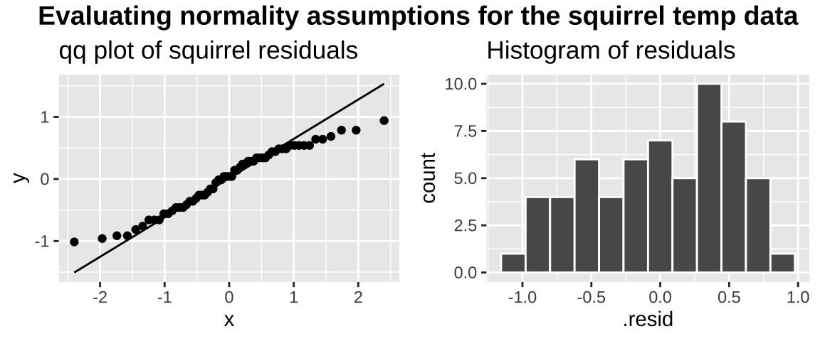
The data are obviously not normal (they look like maybe a uniform), as the small values are too big (above the qq line) and the big values too small (below the qq line) . But the sample size is pretty big, so I would feel comfortable assuming normality here.
25.6 Alternatives to an ANOVA
If you think data do not meet assumptions you can
- Consider this as a caveat when discussing your results, and think through how it could impact your inference.
- Find a more appropriate test.
- Write down your own likelihood function and conduct a likelihood ratio test.
- Permute (but beware)
25.6.1 Permuting as an alternative to the ANOVA based p-value
If we violate the assumption of normal residuals we can permute our data and calculate F, and compare the observed F to its permuted distribution.
The example below is silly because
- The central limit theorem should make our assumptions ok and
- It’s hard to imagine a slight deviation from normality resulting in a p-value of \(10^{-53}\)
But, I’m providing it to show you some fun tricks
n_reps <- 1000

obs_f  <- glance(sqrl_lm) %>%
  pull(statistic)

perm_anova <- sqrl %>%
  rep_sample_n(size = nrow(sqrl), replace = FALSE, reps = n_reps)     %>% # copy the data
  mutate(ambient_temp = sample(ambient_temp, replace = FALSE))        %>% # shuffle labels
  nest(data = c(ambient_temp, body_temp))                             %>% # prepping data for many linear models
  mutate(fit = map(.x = data, ~ lm(.x$body_temp ~ .x$ambient_temp )),     # running many linear models -- one for each permutatatin
         results = map(fit, glance))                                  %>% # turn results into a tibble with glance()
  unnest(results)                                                     %>% #  make results easier to read
  ungroup()                                                           %>%
  dplyr::select(statistic)                                            %>% # grab the F value from permuted data
  mutate(as_or_more = statistic >= obs_f)                             %>%
summarise(p_val = mean(as_or_more))25.7 Post-hoc tests and significance groups
So if we find that not all groups have the same mean, how do we know which means differ? The answer is in a “post-hoc test”. We do a post-hoc test if we reject the null.
I first focus on “unplanned comparisons”, in which we look at all pairs of groups, with no preconception of which may differ.
25.7.1 Unplanned comparisons
Post-hoc test gets over the multiple comparisons problem by conditioning on there being at least one difference and numerous pairwise tests, and altering its sampling distribution accordingly,
The Tukey-Kramer method, with test stat \(q = \frac{Y_i-Y_j}{SE}\), where \(SE = \sqrt{MS_{error}(\frac{1}{n_i}+ \frac{1}{n_j})}\) is one common approach to conduct unplanned post-hoc tests.
To do this in R, we
- Need to run our anova slightly differently, using the
aov()function instead oflm()to make our model.
- Pipe that output to the TukeyHSD() function
aov( body_temp ~ ambient_temp, data = sqrl) %>%
  TukeyHSD()                                %>%
tidy() %>% mutate(adj.p.value = paste(round(adj.p.value * 10^11, digits = 3),"x10^-11",sep = ""))%>% kable(digits = 4)| term | contrast | null.value | estimate | conf.low | conf.high | adj.p.value |
|---|---|---|---|---|---|---|
| ambient_temp | warm-cold | 0 | 6.2543 | 5.8653 | 6.6433 | 1.49x10^-11 |
| ambient_temp | hot-cold | 0 | 10.0000 | 9.6063 | 10.3937 | 1.49x10^-11 |
| ambient_temp | hot-warm | 0 | 3.7457 | 3.3567 | 4.1347 | 1.49x10^-11 |
We find that all pairwise comparisons differ. So we assign cold to significance group A, warm to significance group B and and Hot to group C.
We usually note significance groups on a plot
ggplot(sqrl, aes(x = ambient_temp, y = body_temp, color  = ambient_temp))+
  geom_jitter(height = 0, width = .2, size = 2, alpha = .35, show.legend = FALSE)+
  stat_summary(fun.data = "mean_cl_normal", geom = "errorbar", width = .2, color = "black")+
  scale_color_manual(values = c("blue", "orange", "red"))+
  geom_text(data = tibble(ambient_temp = c("cold","warm","hot"),
                          body_temp     = c(31,37,41),
                          sig_group    = c("a","b","c")),
            aes(label = sig_group), nudge_x = .35, fontface = "bold", show.legend = FALSE)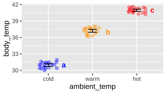
Note significance groupings can be more challenging. For example,
If there was a treatment that for a “very cold” ambient temperature that did not significantly differ from “cold” it would also be in significance group a.
If there was a treatment that for a “balmy” ambient temperature (between warm and hot) that did not significantly differ significantly from warm or hot, it would be in significance groups b and c.