Chapter 36 Generalized linear models I: Yes/No
Motivating scenario: We want to model nonlinear data. Here we use yes/no (or proportion) data as an example.
36.1 Review
36.1.1 Linear models and their asumptions
A statistical model describes the predicted value of a response variable as a function of one or more explanatory variables.
A linear model predicts the response variable by adding up all components of the model. So, In a linear model, we predict the value of a response variable, \(\widehat{Y_i}\) knowing that the observed value, \(Y_i\) will deviate from this prediction by some normally distributed “residual” value, \(e_i\).
\[Y_i = \widehat{Y_i} -e_i\]
We predict Y as a deviation from some constant, a, as a function of a bunch of stuff.
\[\widehat{Y_i} = a + b_1 \times y_{1,i} + b_2 \times y_{2,i} + \dots\]
36.1.1.1 Assumptions of Linear Models
Linear models assume
- Data points are independent.
- Data are unbiased.
- Error is independent of predictors.
- The variance of residuals is independent of predictors.
- Error is normally distributed.
- Response can be modeled as a linear combination of predictors.
36.1.1.2 When data do not meet assumptions
If data do not meet assumptions, we can forge ahead (if the test will be robust), permute/bootstrap, transform, or find a better model.
36.1.1.3 Common violations
We know that a lot of real-world data can be modeled by a linear model, and we also know that the linear model is relatively robust to violations of its assumptions.
Still, there are some relatively violations of assumptions of linear models that are particularly common, especially in biological data.
How biology breaks assumptions of the linear model (better approach in parentheses):
- Heteroscedastic residuals (Use Generalized Least Squares).
- Binomial data (Logistic regression, a generalized linear model for binomially distributed data).
- Count Data (Use a generalized linear model with Poisson, quasi-poison, or negative binomial distributions).
- Non-independence from nested designs. (Mixed effect models).
36.1.2 Likelihood-Based Inference
In Chapter 34, we introduced the idea of likelihood-based inference, which we can use to infer parameters, estimate uncertainty, and test null hypotheses for any data, so long as we can write down a model that appropriately models it.
In Chapter 34, we used this for our familiar linear models. Here, we’ll show the true strength of likelihood-based inference – its flexibility.
36.2 Generalized Linear Models
Generalized Linear Models (GLMs) allow us to model non-linear data by modeling data the way it is distributed. They do so by:
- Specifying the distribution family they come from (the random component).
- Finding a “linear predictor” (systematic component).
- Using a link function to translate from linear predictor to the data.
What does this mean? Let’s look at the example below to clarify!
36.3 GLM Example 1: “logistic regression”
A particularly common type of biological data is yes / no data. Common examples of yes / no data are
- Alive / Dead
- Healthy / Sick
- Present / Absent
- Mated / Unmated
- etc
Such data are poorly described by a standard linear model, but can be modeled. Logistic regression models a yes/no outcome as a function of a continuous predictor (e.g. win/lose, live/die, presence/absence). The linear predictor is the familiar regression equation:
\[\widehat{Y_i} = a + b_1 \times y_{1,i} + b_2 \times y_{2,i} + \dots\]
\(\widehat{Y_i}\) is not our prediction for the probability of “yes”, \(\widehat{p_i}\). Rather, in a GLM, we use this “linear predictor” through the “link function” to find our prediction.
For a logistic regression, the “linear predictor” describes the log odds, which we can convert to the predicted probability of success, \(\widehat{p_i}\) with the logit link function. That is,
\[\widehat{p_i} = \frac{e^{Y_i}}{1+e^{Y_i}}\]
So if our link function says that the log-odds, \(\widehat{Y_i}\), equals negative one, the probability of “yes” is \(\frac{e^{-1}}{1+e^{-1}} = 0.269\). We can find this in R as
exp(-1)/ (1+exp(-1))= 0.269
- Or, more simply, with the
plogis()function.plogis(-1)= 0.269.
36.4 Logistic Regression Example: Cold fish
How does the length of exposure to cold water impact fish mortality? fish survive in cold weather?
Pitkow et al (1960) exposed guppies to 2, 8, 12, or 18 minutes in 5 degree Celsius water. The data – with a value of 1 for Alive meaning alive and a value of zero meaning dead – are presented below
cold.fish <- tibble(Time  = rep(c(2,8,12,18), times = 2),
                    Alive = rep(c(0,1), each = 4),
                    n     = c(11, 24, 29, 38, 29, 16, 11, 2)) %>%
  uncount(weights = n)
What to do??
36.4.1 (Imperfect) option 1: Linear model with zero / one data
We could build a linear model in which we predict survival as a function of time in cold water.
ggplot(cold.fish, aes(x = Time, y = Alive)) +
  geom_jitter(size = 2, alpha = .35, height = .05, width = .5)+
  geom_smooth(method = "lm")+
  scale_x_continuous(breaks = seq(2,18,6),limits = c(0,20))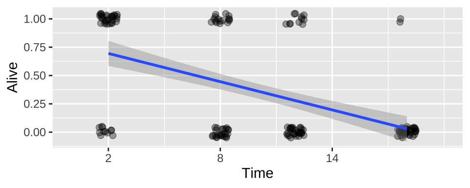
lm_cold_fish1 <- lm(Alive ~ Time, data = cold.fish)
summary.lm(lm_cold_fish1)
##
## Call:
## lm(formula = Alive ~ Time, data = cold.fish)
##
## Residuals:
## Min 1Q Median 3Q Max
## -0.69485 -0.27941 -0.03015 0.30515 0.96985
##
## Coefficients:
## Estimate Std. Error t value Pr(>|t|)
## (Intercept) 0.777941 0.065580 11.863 < 2e-16 ***
## Time -0.041544 0.005665 -7.333 1.1e-11 ***
## ---
## Signif. codes: 0 '***' 0.001 '**' 0.01 '*' 0.05 '.' 0.1 ' ' 1
##
## Residual standard error: 0.4178 on 158 degrees of freedom
## Multiple R-squared: 0.2539, Adjusted R-squared: 0.2492
## F-statistic: 53.78 on 1 and 158 DF, p-value: 1.101e-11We see – unsurprisingly, that fish survival strongly and significantly decreases, the longer they are in cold water.
autoplot(lm_cold_fish1 , ncol = 4)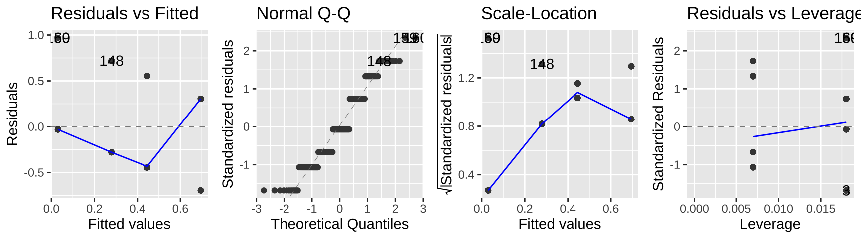
While this isn’t terrible, we do so greatest residuals for intermediate predictions, and the small values are too big (above the xy line) and large values are too big.
So, this isn’t the end of the world, but isn’t ideal.
36.4.2 (Imperfect) option 2: Linear model with proportions
Alternatively, we could convert data to proportions and run a linear model.
cold.fish.summary <- cold.fish %>%
    group_by(Time, Alive) %>%
    summarise(n = n())    %>%
    mutate(n_tot = sum(n),
           prop_survive = n /n_tot)  %>%
    filter(Alive == 1) %>%
ungroup()| Time | Alive | n | n_tot | prop_survive |
|---|---|---|---|---|
| 2 | 1 | 29 | 40 | 0.725 |
| 8 | 1 | 16 | 40 | 0.400 |
| 12 | 1 | 11 | 40 | 0.275 |
| 18 | 1 | 2 | 40 | 0.050 |
lm_cold_fish2 <- lm(prop_survive ~ Time, cold.fish.summary)
summary.lm(lm_cold_fish2)
##
## Call:
## lm(formula = prop_survive ~ Time, data = cold.fish.summary)
##
## Residuals:
## 1 2 3 4
## 0.030147 -0.045588 -0.004412 0.019853
##
## Coefficients:
## Estimate Std. Error t value Pr(>|t|)
## (Intercept) 0.777941 0.040931 19.01 0.00276 **
## Time -0.041544 0.003536 -11.75 0.00717 **
## ---
## Signif. codes: 0 '***' 0.001 '**' 0.01 '*' 0.05 '.' 0.1 ' ' 1
##
## Residual standard error: 0.04124 on 2 degrees of freedom
## Multiple R-squared: 0.9857, Adjusted R-squared: 0.9786
## F-statistic: 138 on 1 and 2 DF, p-value: 0.007166We see – unsurprisingly, that fish survival strongly and significantly decreases (although the p-value is considerably greater than above), the longer they are in cold water.
autoplot(lm_cold_fish2, ncol = 4)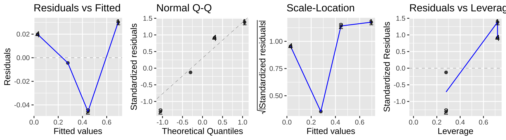
In this case the data seem to meet assumptions, but often they will not. In this case, a bigger issue is that we gave up a ton of power – we went from 160 to four data points. look ok…
36.4.3 (Better) option three – logistic regression
A better option is to model the data as they are – 160 observations of Alive or Dead with forty fish at four different temperatures.
36.4.3.1 Fitting the model
In R, do this with the glm() function, noting that the data are binomially distributed and that we want our link function to be the logit.
There are two equivalent ways to do this.
- For the initial data as zero / one we type
cold.fish.glm1 <- glm(prop_survive ~ Time, weights = n_tot,
data = cold.fish.summary, family = binomial(link = "logit"))- For proportion data we just tell R we want to weight the proportion by the total number of observations for a given X.
cold.fish.glm2 <- glm(prop_survive ~ Time,
                       weights = n_tot, data = cold.fish.summary,
                       family = binomial(link = "logit"))
Regardless, we get the same result for our estimates (and p-values). As in a linear model, we pay attention to the estimates but ignore the incorrect p-values below, and find the correct values with the anova function (see below).
summary.glm(cold.fish.glm1)##
## Call:
## glm(formula = prop_survive ~ Time, family = binomial(link = "logit"),
## data = cold.fish.summary, weights = n_tot)
##
## Deviance Residuals:
## 1 2 3 4
## -0.08866 -0.23245 0.68929 -0.57780
##
## Coefficients:
## Estimate Std. Error z value Pr(>|z|)
## (Intercept) 1.44470 0.37462 3.856 0.000115 ***
## Time -0.22191 0.03886 -5.711 1.12e-08 ***
## ---
## Signif. codes: 0 '***' 0.001 '**' 0.01 '*' 0.05 '.' 0.1 ' ' 1
##
## (Dispersion parameter for binomial family taken to be 1)
##
## Null deviance: 45.72062 on 3 degrees of freedom
## Residual deviance: 0.87086 on 2 degrees of freedom
## AIC: 19.408
##
## Number of Fisher Scoring iterations: 436.4.3.2 Making predictions from the link function
How can we take this output and predict the proportion of fish that will survive exposure to 4C water for some time? Say 6 minutes?
- We first use the linear predictor, to predict the log odds
\[\widehat{Y_i} = 1.44470 -0.22191 \times Time\]
So we predict the log odds of a fish surviving following six minutes of exposure to 4C water to equal \(1.44470 - 6 \times 0.22191 = 0.11324\).
This does not mean that a fish has a 0.11324 probability of surviving six minutes of exposure to 4C water – this is just the log-odds of surviving.
We convert this to a survival probability with the logit link function.
\[p_\text{survive six min} = \frac{e^{0.11324}}{1+e^{0.11324}} = 0.528\]
Or with plogis(), plogis(.11324) = 0.5282798.
This prediction – that a fish at 4C for six minutes has a 52.8% chance of surviving is in line with our plots while incorrectly interpreting the output of the linear predictor as the predicted proportion is not.
36.4.3.3 Testing the model
We formally test the null hypothesis by conducting a likelihood ratio test – that is, we take two times the difference in log-likelihoods and compare this value to its null sampling distribution (which happens to be a \(\chi^2\) distribution with degrees of freedom equal to the difference in the number of parameters estimated for the null and the fitted model).
We can do this with the anova function, telling R tht we want our test tb be the LRT (we get the same answer if we ask or a Chisq).
anova(cold.fish.glm1, test = "LRT")## Analysis of Deviance Table
##
## Model: binomial, link: logit
##
## Response: prop_survive
##
## Terms added sequentially (first to last)
##
##
## Df Deviance Resid. Df Resid. Dev Pr(>Chi)
## NULL 3 45.721
## Time 1 44.85 2 0.871 2.127e-11 ***
## ---
## Signif. codes: 0 '***' 0.001 '**' 0.01 '*' 0.05 '.' 0.1 ' ' 136.4.3.4 Plotting the model
We can add this fit to a plot!!!
For either the raw data
ggplot(cold.fish, aes(x = Time, y = Alive)) +
  geom_jitter(size = 2, alpha = .35, height = .05, width = .5)+
  geom_smooth(method = "glm",method.args = list('binomial'))+
  scale_x_continuous(breaks = seq(2,18,6),limits = c(0,20))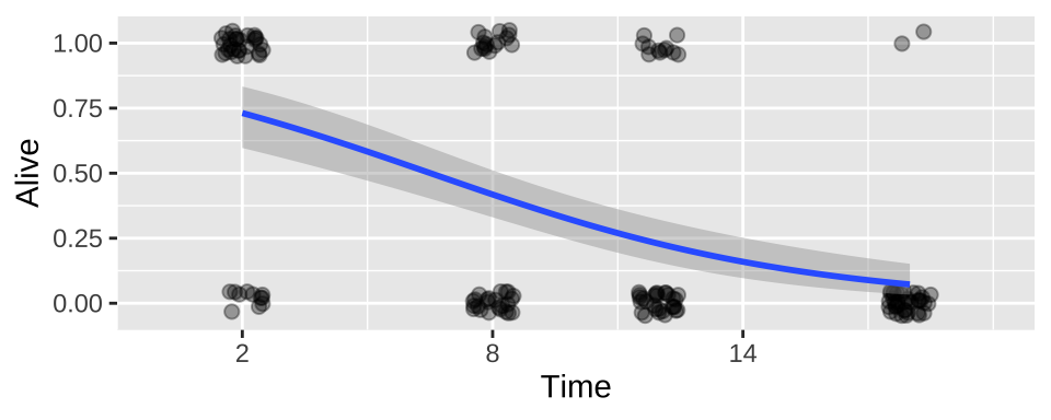
Or the summary
ggplot(cold.fish.summary, aes(x = Time, y = prop_survive, weight = n_tot)) +
  geom_point(size = 2)+
  geom_smooth(method = "glm",method.args = list('binomial'))+
  scale_x_continuous(breaks = seq(2,18,6),limits = c(0,20))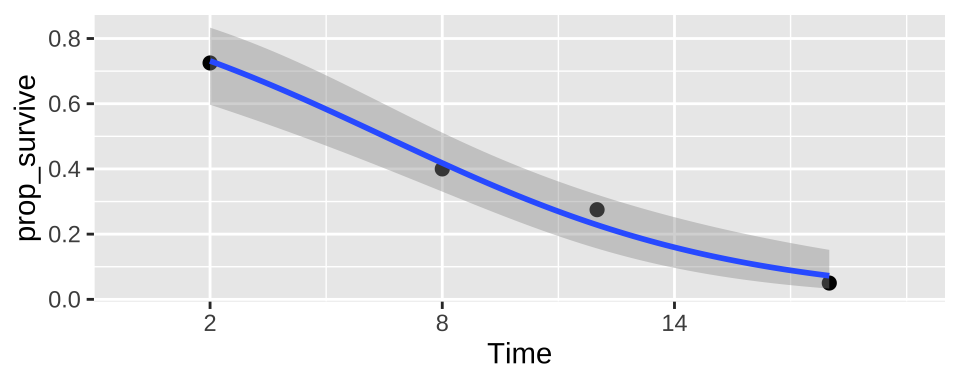
36.4.4 Assumptions of generalized linear models
GLMs are flexible and allow us to model just about anything. But our models must be appropriate for our data. Specifically, GLMs assume
- The data are independently distributed, conditional on predictors (unless this is modeled).
- The residuals are appropriately modelled by the chosen distribution.
- A linear relationship between the transformed response in terms of the link function and the explanatory variables.
- Samples aren’t too small.
36.6 Advanced / under the hood.
36.6.1 How did we find the maximum likelihood?
A straightforward but computationally intense way is a grid search. Here we look over a bunch of parameter combinations and then find the one with the largest log likelihood. R uses more efficient methods to basically do the same thing.
Here’s how we can do this
- Propose a bunch of plausible parameter values (aka models)
models <- crossing(intercept = seq(-2, 2, 0.025),
                   slope     = seq(-.5,.5, .01)) %>%
mutate(model = 1:n())- Evaluate the log-liklihood of each model given the data.
fishLogLik <- function(slope, intercept, dat){
    model_log_lik <- dat %>%
    mutate(p = plogis(intercept + slope * Time),
           logLik = dbinom(x = Alive, size = 1, prob = p, log = TRUE)) %>%
    summarise(sum(logLik)) %>%
    pull()
  return(model_log_lik)
}

models_logLiks <- models %>%
  nest(params = c(intercept, slope)) %>%
  mutate(log_lik = purrr::map_dbl(.x = params, ~ fishLogLik(slope = .x$slope,
                                                   intercept = .x$intercept,
                                                   dat = cold.fish)))%>%
unnest(cols = c(params)) - Find the MLE as the proposed parameters with the greatest log likelihood
top_n(models_logLiks, log_lik, n=1) %>% kable()| model | intercept | slope | log_lik |
|---|---|---|---|
| 13866 | 1.425 | -0.22 | -82.35143 |
Reasuringly, this matches R’s answer.
- We can also use this output to plot a likelihood surface
ggplot(models_logLiks, aes(x = slope, y = intercept, fill = log_lik))+
  geom_tile()+
  scale_fill_gradientn(colours = terrain.colors(500))+
  geom_text(data = . %>% top_n(log_lik, n=1), aes(label = "* MLE"),
            hjust = 0, color = "red")+
  theme_tufte()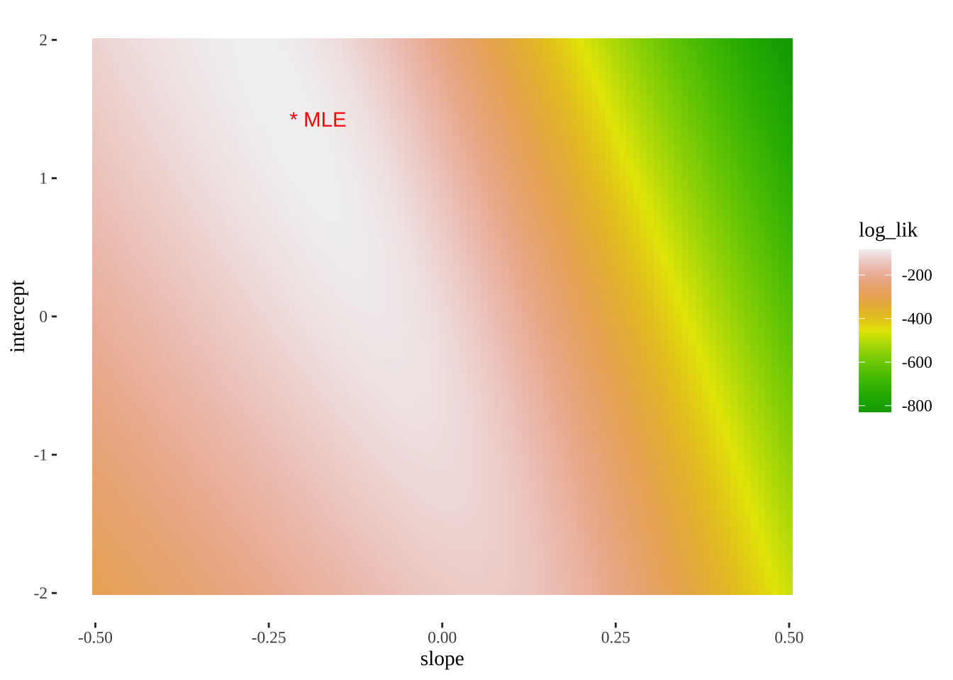
- Finally, we can compare the logLikihood of this model (our best) which equals -82.35143 to the one where we just take the overal mean proportion
cold.fish %>%
    mutate(logLik = dbinom(x = Alive, size = 1,
                           prob =  summarise(cold.fish, mean(Alive)) %>% pull(),
                           log = TRUE)) %>%
    summarise(sum(logLik)) %>%
  pull()
## [1] -104.7749So D = 2* (-82.35143 - (-104.7749)) = 44.84694, and our p-value is pchisq(q = 44.84694, df = 1, lower.tail = FALSE) = 2.1305356^{-11}, which is basically our answer above, save minor rounding error!