Chapter 38 Random effects
Motivating scenario: We want to estimate the variability among groups or the repeatability within subjects, or we want to include nonindependence in our model.
38.1 Review
38.1.1 Linear models
Remember, linear models predict Y as a deviation from some constant, a, as a function of a bunch of stuff.
\[\widehat{Y_i} = a + b_1 \times y_{1,i} + b_2 \times y_{2,i} + \dots\]
38.1.2 Analysis of Variance (ANOVA)
We can test for the significance of factors in linear model in an ANOVA framework.
In Chapter 25, we saw that the total estimate of the variance among groups included that attributable to true differences between groups and those attributable to random sampling error.
Both of these measures go into \(MS_{groups}\) but we expect that that induced by sampling will be roughly equal to \(MS_{error}\).
This is why we test the one-tailed null hypothesis that F (i.e. \(\frac{MS_{groups}}{MS_{error}}\)) equals one, when we ask if the variance among groups is non zero.
38.1.2.1 Assumptions & Common Violations of Linear models
Linear models assume that: (1) Data points are independent, and (2) unbiased, and can be modeled as a linear combination of predictors. With (3) error with a mean and variance that is independent of predictors (4) and normally distributed.
Biology breaks assumptions of the linear models
We have addressed binomial and count data with Logistic and Poisson regression from the generalized linear model.
We are now moving towards addressing what to do when we violate the assumption of independence. This is important because this is among the most commonly broken assumptions in biological data.
38.2 Intro to Random effects
In biology we are rarely interested in specific individuals. Rather we are often interested in variability. Variability over space, or individuals etc.
For example, the response to natural selection depends critical on the genetic variability a population.
In addition to the biological importance of variability, we are often interested as scientists in how repeatable (or reliable) someone is. For example, if we measure the same individual twice how similar will our measurements be relative to the variability in our broader sample.
Finally, sometimes we don’t even care specifically about this variability, but rather we think it will make our data non-independent. For example, if I grow plant in a bunch of plots and want to see the effect of fertilizer on plant growth, I want to model the non-independence of plants in a plot.
All the examples above have something in common – we don’t care about specific individuals or locations, rather we want to know about the variability across them.
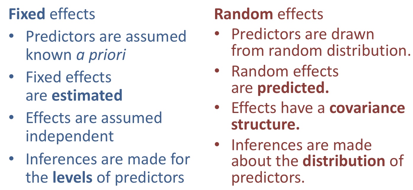
38.2.1 Fixed vs random effects
Up to this point we have considered “fixed effects” e.g. fertilizer choice, experimental treatment etc… For these cases, we want to predict the effects of these treatments, and we don’t generalize to other treatments – for example if I looked at how three fertilizers of interest impacted plant growth, I wouldn’t go and predict the effect of a totally different fertilizer I hadn’t seen before.
However, in the examples above, we did not care about the “fixed effect”. Rather, we were interested in random effects the variability we find across “random” individuals (or locations etc.) in our population. For these cases, we don’t aim to predict the value of individuals, but rather we aim to describe the expected variability we expect across random individuals in our population. Thus, we hope to generalize to a larger population of sample units.
38.2.1.1 How do we know if we have a fixed or random effect?
Some is inherent to the experimental design:
- Are levels of a predictor chosen intentionally (e.g. temperature treatments)? Fixed
- Do we want to make inferences about the levels of a predictor (e.g. mean separation)? Fixed
- Can we reasonably expect covariance between levels of a predictor? Random
Some of this is inherent to the predictor:
- Are the levels of a predictor sampled from some distribution of possible levels? Random
- Can we borrow information across levels of a predictor? Random

38.3 Motivating Example:
Huey and Dunham (1987) were interested in the variability of running speed of the lizard Sceloporus merriam in Big Bend National Park in Texas. So, they built a a two meter raceway, grabbed some lizards and measured their speed. But they were concerned that this would measure something about the lizards motivation to run or the speed at that time etc… so they replicate this and ran each lizard twice.
The data, presented below, can be accessed from this link
38.4 Estimating variance components
ggplot(lizard_runs, aes(x = factor(lizard), y = speed, group = lizard)) +
  geom_point()+
  geom_line()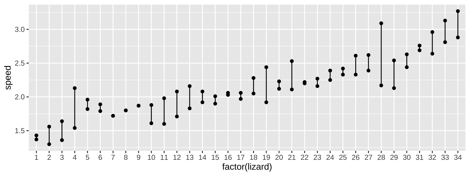
With random effects, we are interested in two sources of variation – that that is between individuals (or locations or whatever) and that that is within them. This sounds a lot like a fixed effects ANOVA, so that will be our starting place. Let’s look at this output, but ignore F and P as we don’t care about them for random effects.
lizard_runs <- lizard_runs %>% mutate( lizard = as.factor(lizard)) # we don't want R thinking lizard 3 is two more than lizard one
lizard_runs_lm <- lm(speed ~ lizard, data = lizard_runs)
anova(lizard_runs_lm)
## Analysis of Variance Table
##
## Response: speed
## Df Sum Sq Mean Sq F value Pr(>F)
## lizard 33 11.3219 0.34309 7.447 3.416e-08 ***
## Residuals 34 1.5664 0.04607
## ---
## Signif. codes: 0 '***' 0.001 '**' 0.01 '*' 0.05 '.' 0.1 ' ' 1We see that the mean squared error (the average squared difference between lizard means and the overall mean) is 0.34309.
Now some of this is due to variability among lizards and some of this is due to chance sampling! How much variability among groups do we expect to arise by chance? – well we know this, it’s the mean squared error!!!!
So, we estimate the variance among groups as this difference divided by the number of individuals per group, because each one contributed to our MS_{group} estimate. Overall, our estimate of the variance among groups, \(s_A^2\) is:
\[s_A^2 = \frac{MS_{group} - MS_{error}}{n_{per group}}\].
For this example, the variance among groups is \(\frac{0.34309 - 0.04607}{2}\) = 0.1485. That is, we think that if we raced each lizard MANY (like an infinite number of) times the variance in average running speeds across lizards would be 0.1485.
38.4.1 With lme4
For simple models like this example, we can use an ANOVA table to estimate \(s_A^2\). But as we get to more complex models that “mix” random and fixed effects this get harder. We can therefore use the lmer() function in the lme4 package to run random and mixed effect (next class) models for us. This syntax of lmer is a lot like lm() with the caveat that we need a language for specifying random effects. We specify that we want to estimate variance (or more precisely standard deviations) in means for a model where groups are random samples from a population as follows
library(lme4) # install lme4 first if you have not already
lizard_runs_rand <- lmer(speed ~ (1|lizard), data = lizard_runs)
lizard_runs_rand
## Linear mixed model fit by REML ['lmerMod']
## Formula: speed ~ (1 | lizard)
## Data: lizard_runs
## REML criterion at convergence: 54.4173
## Random effects:
## Groups Name Std.Dev.
## lizard (Intercept) 0.3854
## Residual 0.2146
## Number of obs: 68, groups: lizard, 34
## Fixed Effects:
## (Intercept)
## 2.139Here
- The “REML criterion at convergence:” is two times the log likelihood of this model
2 * logLik(lizard_runs_rand)=r2 * logLik(lizard_runs_rand) %>% as.numeric()`.
- The
Std.Devfor lizard is the square root of our estimate of the variance among lizards, \(s_A^2\), above (\(\sqrt{0.1485} = 0.385357\)).
- The
Std.DevResidual our estimate for the expected variability within groups is the square root of the mean square error, above (\(\sqrt{0.04607} = 0.2146\)).
- The Fixed effect for the overall intercept is our guess at the mean:
summarize(lizard_runs, mean(speed))= 2.1391176.
38.5 Hypothesis testing for random effects
We can use a likelihood ration test to test the null hypothesis that the among subject variance is zero. We do this by
- Finding two times the difference in log likelihoods of the random effects and null models
- Comparing this value to the \(\chi^2\) distribution with one degree of freedom (because we only estimate one parameter – the variance).
- Because we use Restricted maximum likelihood - (REML) to fit the random effects model, we need to calculate the log likelihood of both the null and random effects model by REML.
log_lik_rand <- lmer(speed  ~ (1|lizard), data = lizard_runs) %>% logLik(REML = TRUE)
log_lik_null <- lm(speed  ~ 1 , data = lizard_runs)           %>% logLik(REML = TRUE)
d <- 2 * (log_lik_rand - log_lik_null)
p <-pchisq(q = d, df = 1, lower.tail = FALSE)
## log_lik_rand log_lik_nul d p
## -2.720865e+01 -4.195827e+01 2.949924e+01 5.593862e-08Or we can have R do this for us with the ranova() function in the lmerTest package
library(lmerTest)
ranova(lizard_runs_rand)
## ANOVA-like table for random-effects: Single term deletions
##
## Model:
## speed ~ (1 | lizard)
## npar logLik AIC LRT Df Pr(>Chisq)
## <none> 3 -27.209 60.417
## (1 | lizard) 2 -41.958 87.917 29.499 1 5.594e-08 ***
## ---
## Signif. codes: 0 '***' 0.001 '**' 0.01 '*' 0.05 '.' 0.1 ' ' 138.6 Repeatability
In a random effects model, we estimate the variance among groups \(s_A^2\). But we might wonder what proportion of the variance in our population do we think is among groups. This is known as “repeatability” or “the interclass correlation” and equals
\[\frac{s_A^2}{s_A^2 + MS_{error}}\]
A repeatability of zero means that measuring the same sample twice is about as reliable as taking two random samples, while a repeatability of one would imply no variation within an individual.
The repeatability for our lizard running example is = 0.763, so this is pretty repeatable.
38.6.1 Repeatability vs \(R^2\)
Repeatability measures how repeatable our measure is – that is what is how similar do we expect two measurements from a random lizard to be. This is only meaningful for random effects, but is super useful because this parameter has meaning outside of our model.
This is very different than \(r^2\) the proportion of variance “explained by our model” (\(SS_{groups}/SS_{total}\)). \(r^2\) is not a parameter we can interpret outside of the scope of a single experiment. In our example \(r^2\) equals \(11.3219 / ( 11.3219 +1.5664) = 0.8785\) a number that clearly differs from our estimated repeatability.
38.7 Shrinkage
We know from our background on “regression to the mean” that exceptional values are likely overestimates. A ice benefit of the random effects approach is that we share information across individuals. That is, our estimate for an individual is “shrunk” towards the overall population mean.
Shrinkage depends on:
- How variable the coefficients are across clusters
- The degree of uncertainty associated with individual estimates
Let’s explore this for our lizard data:
First, lets grab predictions from our fixed effect model
fixed_predicted_means <- augment(lizard_runs_lm) %>%
  dplyr::select(lizard, .fitted) %>%
  dplyr::distinct(lizard,.fitted)%>%
  mutate(effect = "fixed")
Now let’s grab predictions from our random effect model
rand_predicted_means <- broom.mixed::augment(lizard_runs_rand) %>%
  dplyr::select(lizard, .fitted) %>%
  dplyr::distinct(lizard,.fitted)%>%
  mutate(effect = "random")
Now let’s combine them and plot. We see this “shrinkage” as extreme estimates are pulled toward the mean in the random-effect based estimates.
bind_rows(fixed_predicted_means,rand_predicted_means) %>%
  mutate(lizard = fct_reorder(lizard, .x = .fitted, .fun = mean)) %>%
  ggplot(aes(x = lizard, y = .fitted, color = effect))+
  geom_point()+
  geom_hline(yintercept =  2.139)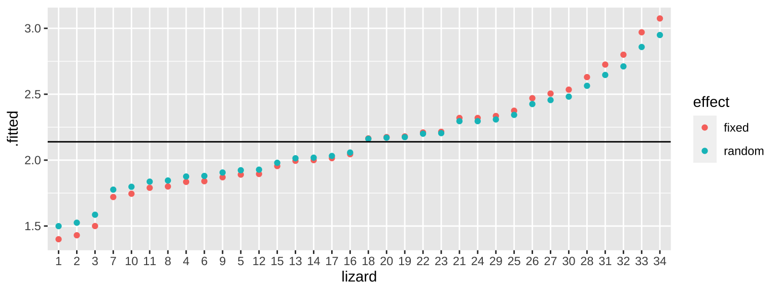
38.8 Assumptions of random effects models
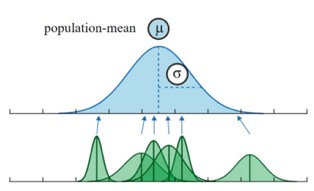
Random effects models make our standard linear model assumptions and also assumes that groups (e.g. individuals, sites, etc.) are sampled at random and that group means are normally distributed.
But, we see in the next chapter that by modeling random effects we can model non-independence of observations.