Chapter 37 Generalized linear models II: Count Data
Motivating scenario: We want to model nonlinear data. Here we use count (or proportion) data as an example.
37.1 Review
37.1.1 Linear models and their asumptions
Remember, linear models predict Y as a deviation from some constant, a, as a function of a bunch of stuff.
\[\widehat{Y_i} = a + b_1 \times y_{1,i} + b_2 \times y_{2,i} + \dots\] and assume that
- Data points are independent.
- Data are unbiased.
- Error is independent of predictors.
- The variance of residuals is independent of predictors.
- Error is normally distributed.
- Response can be modeled as a linear combination of predictors.
37.1.1.1 Common violations
How biology breaks assumptions of the linear model (better approach in parentheses):
- Heteroscedastic residuals (Use Generalized Least Squares).
- Binomial data (Logistic regression, a generalized linear model for binomially distributed data).
- Count Data (Use a generalized linear model with Poisson, quasi-poison, or negative binomial distributions).
- Non-independence from nested designs. (Mixed effect models).
37.1.2 Likelihood-Based Inference
In Chapter 34, we introduced the idea of likelihood-based inference, which we can use to infer parameters, estimate uncertainty, and test null hypotheses for any data, so long as we can write down a model that appropriately models it
37.2 Generalized Linear Models
Generalized Linear Models (GLMs) allow us to model non-linear data by modeling data the way it is distributed. In chapter 36, we modelled yes/no data with a logistic regression.
Recall that GLMs we:
- Specify the distribution family they come from (random component).
- Find a “linear predictor” (systematic component).
- Use a link function to translate from linear predictor to the scale of data.
37.3 GLM Example 2: “Poisson regression” and count data
A particularly common type of biological data is count data. Common examples of count data are
- Number of mating attempts.
- Number of mutation (or recombination) events.
- Number of individuals in a plot.
- etc
Such data are poorly described by a standard linear model, but can be modeled. Below, I simulate leaves falling randomly on a landscape. We see that the number of leaves in each quadrant does not follow a normal distribution.
sim_rand_location <- tibble(x = runif(110), y = runif(110)) %>%
  mutate(x_box = cut(x, breaks = seq(0,1,.1)),
         y_box = cut(y, breaks = seq(0,1,.1)))

plot_location <- ggplot(sim_rand_location , aes(x = x, y = y, label = emoji("fallen_leaf"))) +
  geom_text(family="EmojiOne", color = "brown", hjust = 0.5, vjust = 0.5)+
  theme_tufte() +  geom_vline(xintercept = seq(0,1,.1), color = "black", alpha = .3)+
  geom_hline(yintercept = seq(0,1,.1), color = "black", alpha = .3)+
  scale_x_continuous(expand = c(0,0)) +    scale_y_continuous(expand = c(0,0))

location_histogram <- sim_rand_location %>%
  group_by(x_box, y_box, .drop = FALSE) %>%
  summarise(n = n())     %>%
  ggplot(aes(x = n))+
  geom_histogram(binwidth = 1, color = "white", size = 2)+
  scale_x_continuous(breaks = seq(0,8,1))+
  theme_light()

plot_grid(plot_location, location_histogram, ncol =2)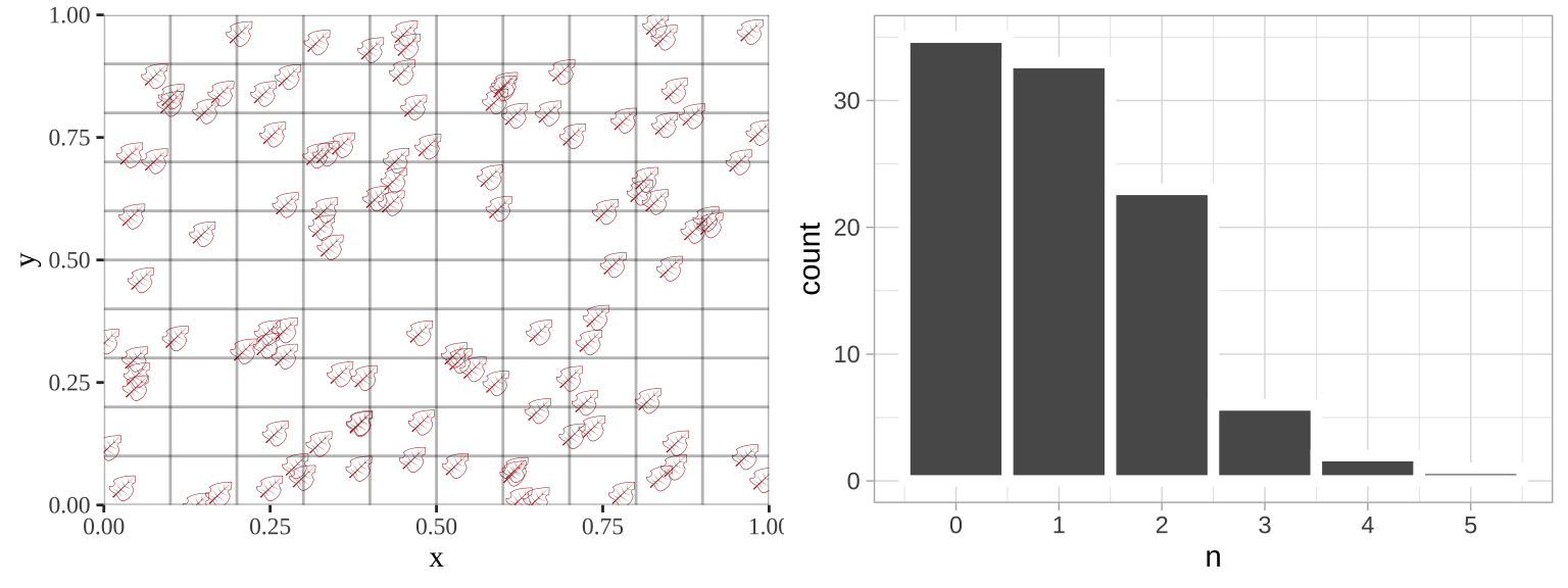
37.3.1 The poisson distribution
If these counts are randomly distributed over time or space, they will follow a Poisson distribution. For this reason, the Poisson is a common starting place for modeling count data.
If there are, on average, \(\lambda\) things per unit of time or space, the poisson equation predicts the probability the we have X things in one unit of time or space equals
\[P(X) = \frac{e^{-\lambda} \lambda^X}{X!}\] The mean of the Poisson is \(\lambda\), as is the variance. Because the variance increases with the mean, Poisson distributed data often violates the homoscedasticity assumption of linear models.
So, for the leaf example, above we have
- 110 leaves land in 100 quadrants of this equally sized 10 x 10 grid.
- So \(\lambda = 110/100\). So we have 1.10 leaves per quadrant.
- The probability that a given quadrant has three leaves equals \(P(3) = \frac{e^{-1.1} 1.1^3}{3!} = 0.0738419\). We can find this in R as
exp(-1.1) * 1.1^3 / factorial(3)= 0.0738419. or more simply, as
dpois(x = 3, lambda = 1.1)= 0.0738419.
- So, we expect \(100 \times 0.0738419 = 7.38\) of the 100 quadrats to have exactly three leaves.
leaves_per_quadrant <- 1.1
n_quadrants         <- 100

expected_leaves <- tibble(n_leaves = 0:6,
       prob_n_leaves = dpois(x = n_leaves, lambda = leaves_per_quadrant),
expected_number_quadrats = n_quadrants * prob_n_leaves)| n_leaves | prob_n_leaves | expected_number_quadrats |
|---|---|---|
| 0 | 0.3328711 | 33.2871084 |
| 1 | 0.3661582 | 36.6158192 |
| 2 | 0.2013870 | 20.1387006 |
| 3 | 0.0738419 | 7.3841902 |
| 4 | 0.0203065 | 2.0306523 |
| 5 | 0.0044674 | 0.4467435 |
| 6 | 0.0008190 | 0.0819030 |
location_histogram +
  geom_line(data = expected_leaves, aes(x = n_leaves , y = expected_number_quadrats), color = "red")+
  annotate(x = 4, y = 30, geom = "text", label = "Poisson\nexpectations", color = "red", hjust = 0)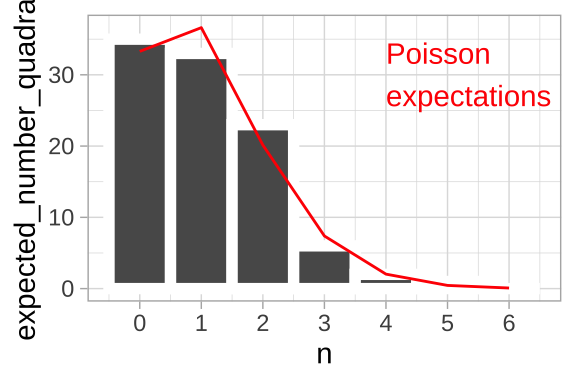
37.3.2 The Poisson regression
The poison regression is a generalized linear model for Poisson distributed data. As in the logistic regression, the linear predictor is the familiar regression equation:
\[\widehat{Y_i} = a + b_1 \times y_{1,i} + b_2 \times y_{2,i} + \dots\]
\(\widehat{Y_i}\) is not our prediction for the count \(\widehat{\lambda_i}\). Rather, in a GLM, we use this “linear predictor” through the “link function” to find our prediction.
For a Poisson regression, the “linear predictor” describes the log of the predicted number, which we can convert to the predicted count by exponentiation. That is,
\[\widehat{\lambda_i} = e^{Y_i}\]
So if our link function says that the log of the expected count, \(\widehat{Y_i}\), equals 3, we expect, on average, a count of \(e^{3} = 20\). We can find this in R as
exp(3)= 20.0855369
37.4 Poisson regression example: Elephent
Do older elephant males have more mates?
elephants <- tibble(mates = c(0,1,1,1,3,0,0,0,2,2,2,1,2,4,3,3, 3,2,1,1,2,3,5,6,1, 1,6,2,1,3,4,0,2,3,4,9,3,5,7,2,9),
                    age = c(27,28,28,28,28,29,29,29,29,29,29,30,32,33,33,33, 33,33,34,34, 34,34,36,36,37,37,37,38,39,41,42,43, 43,43,43,43,44,45,47,48,52))
37.4.1 (Imperfect) Option 1: Linear model on raw data
ggplot(elephants, aes(x = age, y = mates, label = emoji("elephant"))) +
  geom_text(family="EmojiOne", color = "black",
            position = position_jitter(width = .1, height = .1))+
  geom_smooth(method = "lm")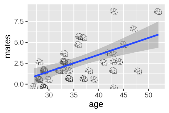
We could simply run a linear regression.
elephant_lm1 <- lm(mates ~ age, data = elephants)
summary(elephant_lm1)
##
## Call:
## lm(formula = mates ~ age, data = elephants)
##
## Residuals:
## Min 1Q Median 3Q Max
## -4.1158 -1.3087 -0.1082 0.8892 4.8842
##
## Coefficients:
## Estimate Std. Error t value Pr(>|t|)
## (Intercept) -4.50589 1.61899 -2.783 0.00826 **
## age 0.20050 0.04443 4.513 5.75e-05 ***
## ---
## Signif. codes: 0 '***' 0.001 '**' 0.01 '*' 0.05 '.' 0.1 ' ' 1
##
## Residual standard error: 1.849 on 39 degrees of freedom
## Multiple R-squared: 0.343, Adjusted R-squared: 0.3262
## F-statistic: 20.36 on 1 and 39 DF, p-value: 5.749e-05Here we estimate that elephant males expect, on avaerage, an additional 0.20 mates (95% CI 0.11, 0.29) for every year they live.
But we can see a few issues in the diagnostic plots – namely, the “scale-location” plot shows that the variance in the residuals increases with the predicted value.
autoplot(elephant_lm1, ncol = 4)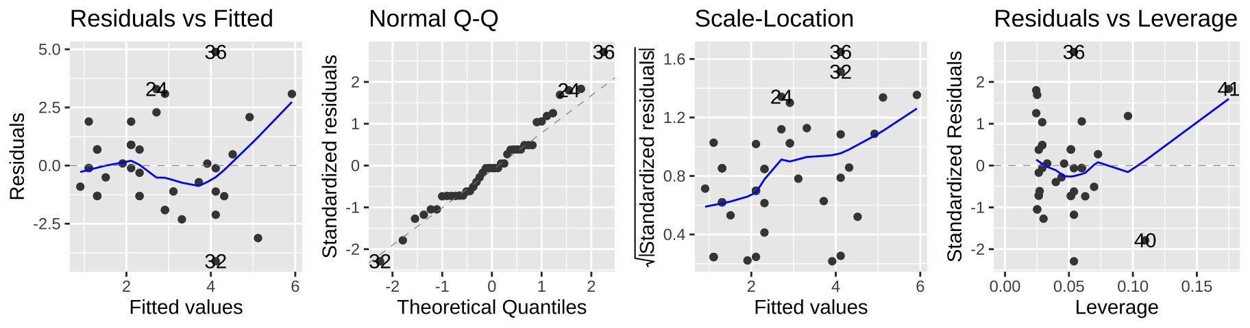
37.4.2 (Imperfect) Option 2: Linear model on log plus one transformed data
ggplot(elephants, aes(x = age, y = mates, label = emoji("elephant"))) +
  geom_text(family="EmojiOne", color = "black",
            position = position_jitter(width = .1, height = .1))+
  geom_smooth(method = "lm")+
  scale_y_continuous(trans = "log1p")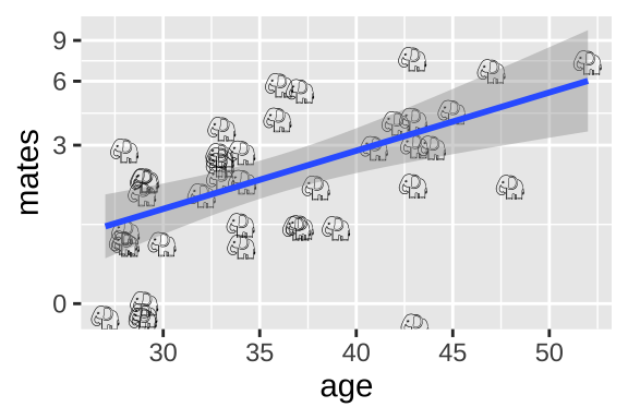
Alternatively, we could add one to the number of maters and then log transfoarm to better meet assumptions of the linear model
elephant_lm2 <- lm(log1p(mates) ~ age, data = elephants)
summary(elephant_lm2)
##
## Call:
## lm(formula = log1p(mates) ~ age, data = elephants)
##
## Residuals:
## Min 1Q Median 3Q Max
## -1.49087 -0.33939 0.06607 0.35376 0.81171
##
## Coefficients:
## Estimate Std. Error t value Pr(>|t|)
## (Intercept) -0.69893 0.45861 -1.524 0.135567
## age 0.05093 0.01259 4.046 0.000238 ***
## ---
## Signif. codes: 0 '***' 0.001 '**' 0.01 '*' 0.05 '.' 0.1 ' ' 1
##
## Residual standard error: 0.5237 on 39 degrees of freedom
## Multiple R-squared: 0.2957, Adjusted R-squared: 0.2776
## F-statistic: 16.37 on 1 and 39 DF, p-value: 0.0002385These model parameters take a minute to interpret – we start with an intercept of -0.69893 and add 0.05093 for each year lived. To turn this into a prediction, we exponentiate ad subtract one. So, for example, we predict that a 40 year old elephant will have \(e^{(-0.69893 + 40 \times 0.05093)}-1 = 2.81\) mates.
autoplot(elephant_lm2, ncol = 4)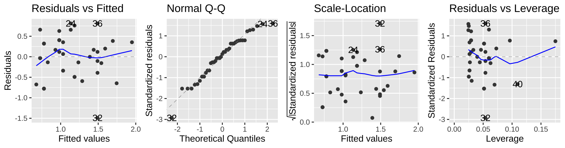
This seems to meet model assumptions pretty well, and is a totally acceptable option – but in a sense, we already dealt with the complexity of transforming our data for the model and then back-transforming to explain the results, so a Poisson regression might be more convenient.
37.4.3 (Better) Option 3: Poisson regression
Rather than transforming the data to fit the test, we can actually model the data we have. We do this with the Poisson Regression.
We model data as being Poisson distributed – that is, we ultimately predict the expected count for a given predictor \(\lambda_i\) assuming Poisson distributed errors. But remember that before that, we find our linear predictor, \(Y_i\), as we do for a standard linear model, and the exponential our prediction, \(Y_i\) to find \(\lambda_i\).
As with the logistic regression (Ch 36), we find the linear predictor with the glm() function. This time, we specify that we are modeling a Poisson random variable with a log link function:
elephant.glm <- glm(mates ~ age, data = elephants, family = poisson(link = "log"))
elephant.glm
##
## Call: glm(formula = mates ~ age, family = poisson(link = "log"), data = elephants)
##
## Coefficients:
## (Intercept) age
## -1.58201 0.06869
##
## Degrees of Freedom: 40 Total (i.e. Null); 39 Residual
## Null Deviance: 75.37
## Residual Deviance: 51.01 AIC: 156.537.4.3.1 Predictions from a poisson regression
So for our linear predictor, we begin with an intercept of -1.582 and add 0.06869 for every year an elephant has lived. So for a 40 year old elephant, the linear predictor, \(Y_{age = 40} = -1.582 + 40 \times 0.06869 = 1.1656\). Exponentiating this (to convert from log to linear scale), we predict that a 40 year old elephant male, will have, on average \(e^{1.1656} = 3.2\) mates (in R exp(1.1656)), with Poisson distributed error.
37.4.3.2 Plotting results of a poisson regression
We can visualize the poisson regression as follows:
ggplot(elephants, aes(x = age, y = mates, label = emoji("elephant"))) +
  geom_text(family="EmojiOne", color = "black",
            position = position_jitter(width = .1, height = .1))+
  geom_smooth(method = "glm",method.args = list('poisson'))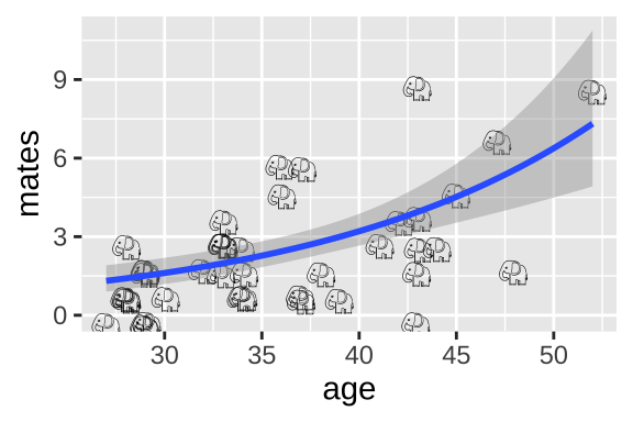
37.4.3.3 Hypothesis testing for a poisson regression
As with the logistic regression (Ch 36), we compare the likelihood of our MLE parameter estimate to a null model with a likelihood ratio test.
We can do this ourselves
null.elephant.glm <- glm(mates ~1, data = elephants, family = poisson(link = "log"))
D                 <- 2 * (logLik(elephant.glm) - logLik(null.elephant.glm))
p.val             <- pchisq(q = D, df = 1, lower.tail = FALSE)
c(D=D, p.val = p.val)
## D p.val
## 2.436011e+01 7.990620e-07Or with the anova() function
anova(elephant.glm, test = "LRT")## Analysis of Deviance Table
##
## Model: poisson, link: log
##
## Response: mates
##
## Terms added sequentially (first to last)
##
##
## Df Deviance Resid. Df Resid. Dev Pr(>Chi)
## NULL 40 75.372
## age 1 24.36 39 51.012 7.991e-07 ***
## ---
## Signif. codes: 0 '***' 0.001 '**' 0.01 '*' 0.05 '.' 0.1 ' ' 1We see that the “deviance” that R calculates is our D, and that our p-values match R’s.
We reject thee null!
An aside on the deviance
If we look at our GLM output, wee see “Null Deviance” and “Reidual Deviance”, with our D eaul to two times their difference.
elephant.glm##
## Call: glm(formula = mates ~ age, family = poisson(link = "log"), data = elephants)
##
## Coefficients:
## (Intercept) age
## -1.58201 0.06869
##
## Degrees of Freedom: 40 Total (i.e. Null); 39 Residual
## Null Deviance: 75.37
## Residual Deviance: 51.01 AIC: 156.5What does this mean?
Well, we first find the log likelihood likelihood of the perfect, “oversaturated” model, for which every prediction is perfect.
oversaturated_elephants <- elephants %>%
  dplyr::select(mates) %>%
  mutate(logLik = dpois(x = mates, lambda = mates, log = TRUE))
So the log likelihood of a perfect model is summarise(oversaturated_elephants, logLik = sum(logLik))
= -50.7230814.
We find the log likelihood of our model is
logLik_elephant_glm <- broom::augment(elephant.glm) %>%
   dplyr::select(mates,   age, .fitted)%>%
    mutate(lambda = exp(.fitted),
logLik = dpois(x = mates, lambda = lambda, log = TRUE))DT::datatable(logLik_elephant_glm %>%
mutate(.fitted = round(.fitted,digits = 3),
lambda = round(lambda, digits = 3),
logLik = round(logLik, digits =3)),
options = list(autoWidth = TRUE,pageLength = 5, lengthMenu = c(5, 25, 50)))So the log likelihood of our model is summarise(logLik_elephant_glm, logLik = sum(logLik))
= -76.2288953, which is what we could have found by logLik(elephant.glm) = -76.2288953.
The “Residual Deviance” is two times the difference in the log likelihood of a perfect model, -50.72308 and our model, -76.2289 – i.e. 2 * ((-50.72308 ) - (-76.2289 )) = 51.01164.
We can then get our “Deviance” of 75.37174 - 51.01164 = 24.3601, which we previously found by simply taking two times the difference in the log likelihood of the MLE and null models.
An aside on residuals
If we look at the residuals of our model, we see something strange…
broom::augment(elephant.glm) It is not the difference between our observation, mates and \(\widehat{Y_i}\), nor is it the difference between our prediction and the predicted \(\lambda_i\) (for example we have zero mates and a prediction of $e^{0.273} = 1.3139. The acutal calculation is a bit obscure, and we won’t adress it here, just know that they should look good on a diagnostic plot, and if they don’t, there may be better options that a Poisson regression.
See this for more background on interpretting residuals from poisson regression.
37.5 Assumptions of poisson regression
Remember that a GLM still makes assumptions and that these assumptions can differ from the of a linear model because we are building a different model.
A poisson regression assumes that
- Poisson Response – that is that the response variable is poisson distributed (for each prediction).
- So, e.g. a continuous response value would not make sense.
- This also implies that the variance for a given value, \(\sigma^2_i\) should equal the mean. \(\lambda_i\).
- So, e.g. a continuous response value would not make sense.
- Independence of responses (conditional on predictors).
- That predictions can be made by adding up elements of the linear predictor and exponentiating.
- That data are collected without bias.
Viewing our standard diagnostic plots can help us evaluate some of these assumptions. As I said above, don’t think too hard about these y-values – think of them as a residual that would look as we hpoe if the model was a good fit.
autoplot(elephant.glm, ncol=4)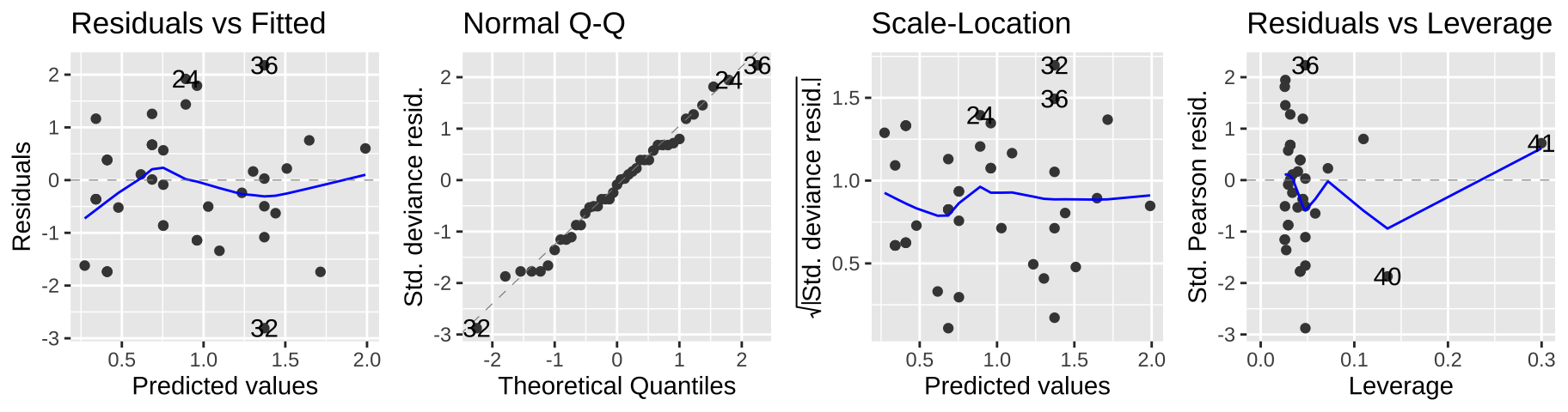
Another rough diagnostic is to look at the “Dispersion” – a measure of how much more variance we see than we expect from a Poisson model. We can approximate this by dividing the Residual deviance by the degrees of freedom.
- A dispersion parameter of one means the variance is well predicted by the Poisson model.
- A dispersion way greater than one (like 2.5 or greater) suggests that a Poisson model is inappropriate.
In our case this is 51.01/40 = 1.275, which is just fine.
37.5.1 Model fit
We can also evaluate if the model is a reasonable description of the data by comparing our likelihoods to the likelihood of data simulated directly from the model.
Let’s make this concretre by simulating once with the rpois() function:
sim1 <- broom::augment(elephant.glm) %>%
  dplyr::select(mates,   age, .fitted) %>%
  mutate(simulated = rpois(n=n(), lambda = exp(.fitted)),
         logLikSim = dpois(x = simulated, lambda = exp(.fitted), log = TRUE))
So the log likelihood of this data set simulaed from our mode is sim1 %>% summarise(sum(logLikSim)) = -78.4351573. Which isn’t far from the likelihood of the the model for the actual data– logLik(elephant.glm) -76.2288953.
If we did a bunch of these simulations and our log likelihood way further from zero than nearly all simulated cases, we’d worry about model fit. The histogram below suggests
# here we write a function to simulate data from a poisson with predictions of a linear model
# and return the log likelihood

simPois <- function(pois.glm){
  broom::augment(pois.glm) %>%
    dplyr::select(.fitted) %>%
    mutate(simulated = rpois(n=n(), lambda = exp(.fitted)),
           logLikSim = dpois(x = simulated, lambda = exp(.fitted), log = TRUE)) %>%
    summarise(loglik = sum(logLikSim)) %>%
    pull()
}


tibble(simLogLiks = replicate(n = 1000, simPois(pois.glm = elephant.glm))) %>% # simulate 1000 times
  ggplot(aes(x = simLogLiks)) +
  geom_histogram(bins = 30)+
  scale_x_reverse()+
  geom_vline(xintercept =  logLik(elephant.glm), color = "red")+
  labs(subtitle = "Comparing the log likelihood with real and simulated data")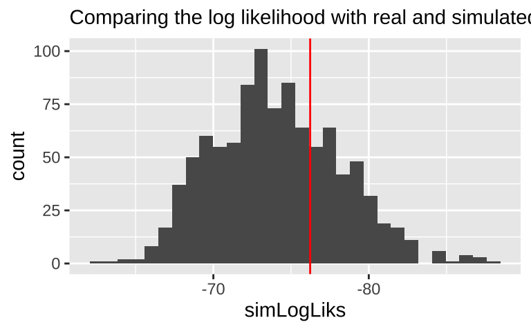
37.6 Alternatives to the poisson regresssion
So, the Poisson is a good model if count data are random over space or time. But sometimes they are not. Common violations of Poisson assumptions include
- Overdispersion (more variance than predicted by the Poisson)
- Zero inflation (too many zeros)
Quasipoisson & beta-binomial are usually good options for modeling overdispersion.
“Hurdle” models can be used to model “zero inflated” data.
37.8 Advanced / under the hood.
37.8.1 How did we find the maximum likelihood?
A straightforward but computationally intense way is a grid search. Here we look over a bunch of parameter combinations and then find the one with the largest log likelihood. R uses more efficient methods to basically do the same thing.
Here’s how we can do this
- Propose a bunch of plausible parameter values (aka models)
models <- crossing(intercept = seq(-3, -1, 0.005),
                   slope     = seq(-0, 0.1, .002)) %>%
mutate(model = 1:n())- Evaluate the log-likelihood of each model given the data.
# write a function to calcualte the likleihoods given a model
elephantLogLik <- function(slope, intercept, dat){
    model_log_lik <- dat %>%
    mutate(p = exp(intercept + slope * age),
           logLik = dpois(x = mates, lambda = p, log = TRUE)) %>%
    summarise(sum(logLik)) %>%
    pull()
  return(model_log_lik)
}

models_logLiks <- models %>%
  nest(params = c(intercept, slope)) %>%
  mutate(log_lik = purrr::map_dbl(.x = params, ~ elephantLogLik(slope = .x$slope,
                                                   intercept = .x$intercept,
                                                   dat = elephants)))%>%
unnest(cols = c(params)) - Find the MLE as the proposed parameters with the greatest log likelihood
top_n(models_logLiks, log_lik, n=1) %>% kable()| model | intercept | slope | log_lik |
|---|---|---|---|
| 14774 | -1.555 | 0.068 | -76.23017 |
Reassuringly, this matches R’s answer.
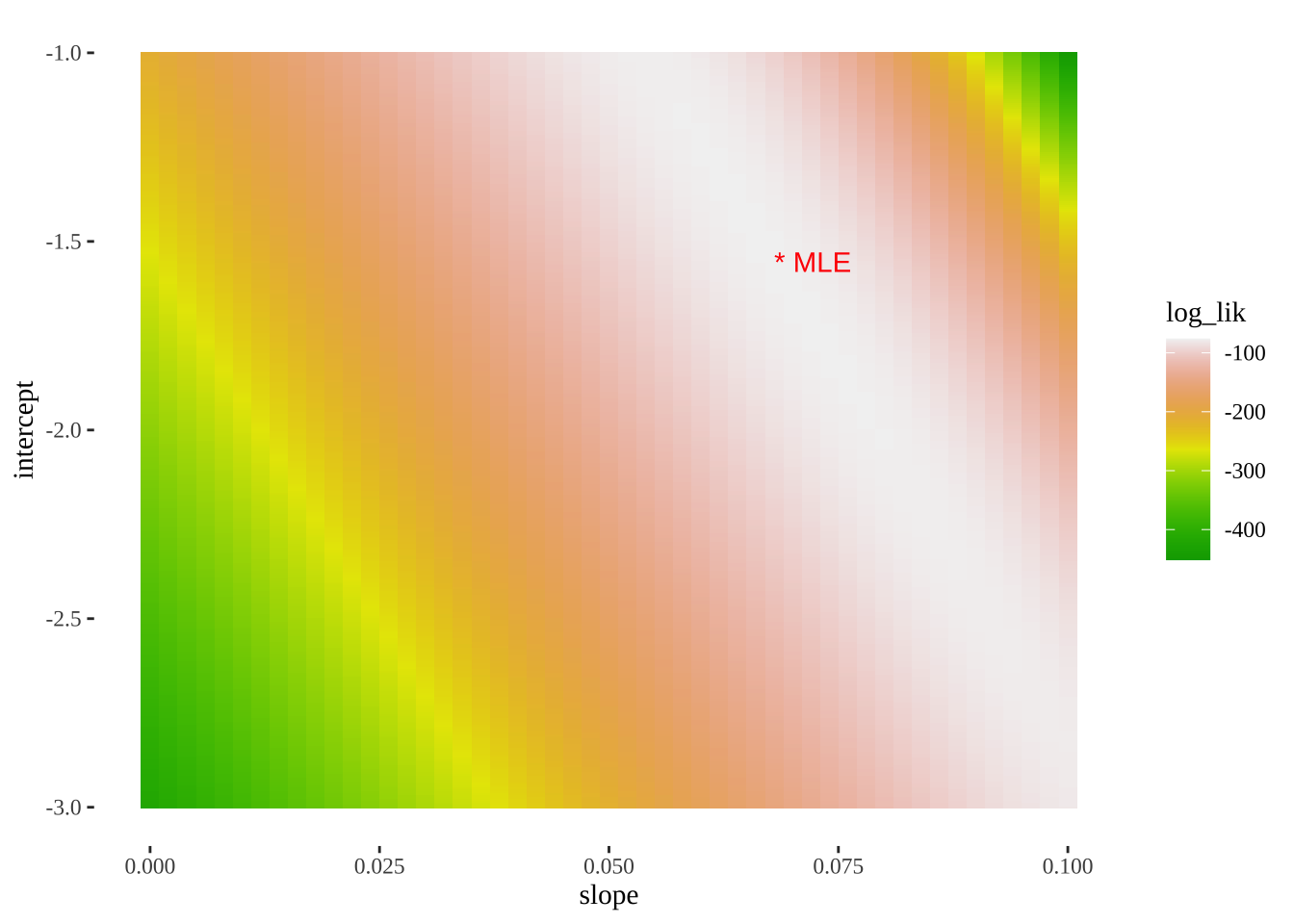
- We can also use this output to plot a likelihood surface
ggplot(models_logLiks, aes(x = slope, y = intercept, fill = log_lik))+
  geom_tile()+
  scale_fill_gradientn(colours = terrain.colors(500))+
  geom_text(data = . %>% top_n(log_lik, n=1), aes(label = "* MLE"),
            hjust = 0, color = "red")+
  theme_tufte()