Chapter 13 Review and reflect on the most important stats concepts we have learned so far
Motivating scenarios: We are hoping to solidify our understanding of concepts foundational to our understanding of statistics.
Learning goals: By the end of this chapter you should be able to Think hard about and explain
- The idea of a population and a parameter.
- The most common parameters we estimate (mean and standard deviation/variance)
- The concept of sampling and the difference between sampling error, sampling bias, and non-independent sampling.
- The sampling distribution.
- The expected standard error of a distribution of some size from a population (connect this to the idea of the sampling distribution).
- How and why we get a sense of the standard error from our sample, and why bootstrapping (kind of) makes sense as a way to do this.
- Why barplots +/- standard errors are not a good way to display continuous variables.
13.1 Questions to consider
To help review think about the following questions:
Statisticians imagine we sample mythical populations with parameters. But basically we never have a population (and they kind of only exist in the imagination of statisticians).
- Why is this a super helpful way to think?
- Why is this a super weird way to think?
- On balance, is the idea of a population a helpful or unhelpful construct?
- Why is this a super helpful way to think?
Say you are interested in comparing COVID outbreaks across state / countries / time What should you worry about more, sampling error or sampling bias?
What is the sampling distribution? How does it relate to the idea of a population? Why do we build a sampling distribution by using the
slice_sample(...), getting a summary stat withsummarize(), and doing this a bunch withreplicate()?- Why do we do this in stats class?
- Why do we not do this with actual data?
- What do we do with actual data that is inspired by this view?
- Why do we do this in stats class?
We use our data to imagine the sampling distribution of the population we think we sampled from (e.g. by bootsrapping, or with math formulas), with the aim of thinking about how far away the estimate from our sample is from the true and unknown population parameter.
- Why is this a nonsensical thing to do?
- Why does it make good sense?
- Which argument do you find more compelling?
- Why is this a nonsensical thing to do?
In class I teach bootstrapping before math to describe uncertainty, while traditionally this is taught in the other order.
- Why do I do this?
- Why is it a good idea?
- Why is it a bad idea?
- On the whole which order would you recommend this approach? Why or why not?
- Why do I do this?
I teach bootstrapping with the
slice_sample(...)function withreplace = TRUE, getting a summary stat withsummarize(), and doing this a bunch withreplicate()to describe uncertainty in our estimate. Alternatively, we could have used the bootstrap function in that package (so we wouldn’t need to specifyreplace = TRUEetc. etc.), or we could have written or own functions. Weigh the pros and cons of each approach… Do you think the way we code this up helps us understand bootstrapping or is that irrelevant?Why is the bootstrap inappropriate for very small sample sizes?
Type the equation for the sample standard deviation here then explain the standard deviation in your own words.
Explain the relationship between the standard deviation and the standard error. Which describes uncertainty and which describes variability? What is the difference? Which one (or any or both) will change with the sample size?
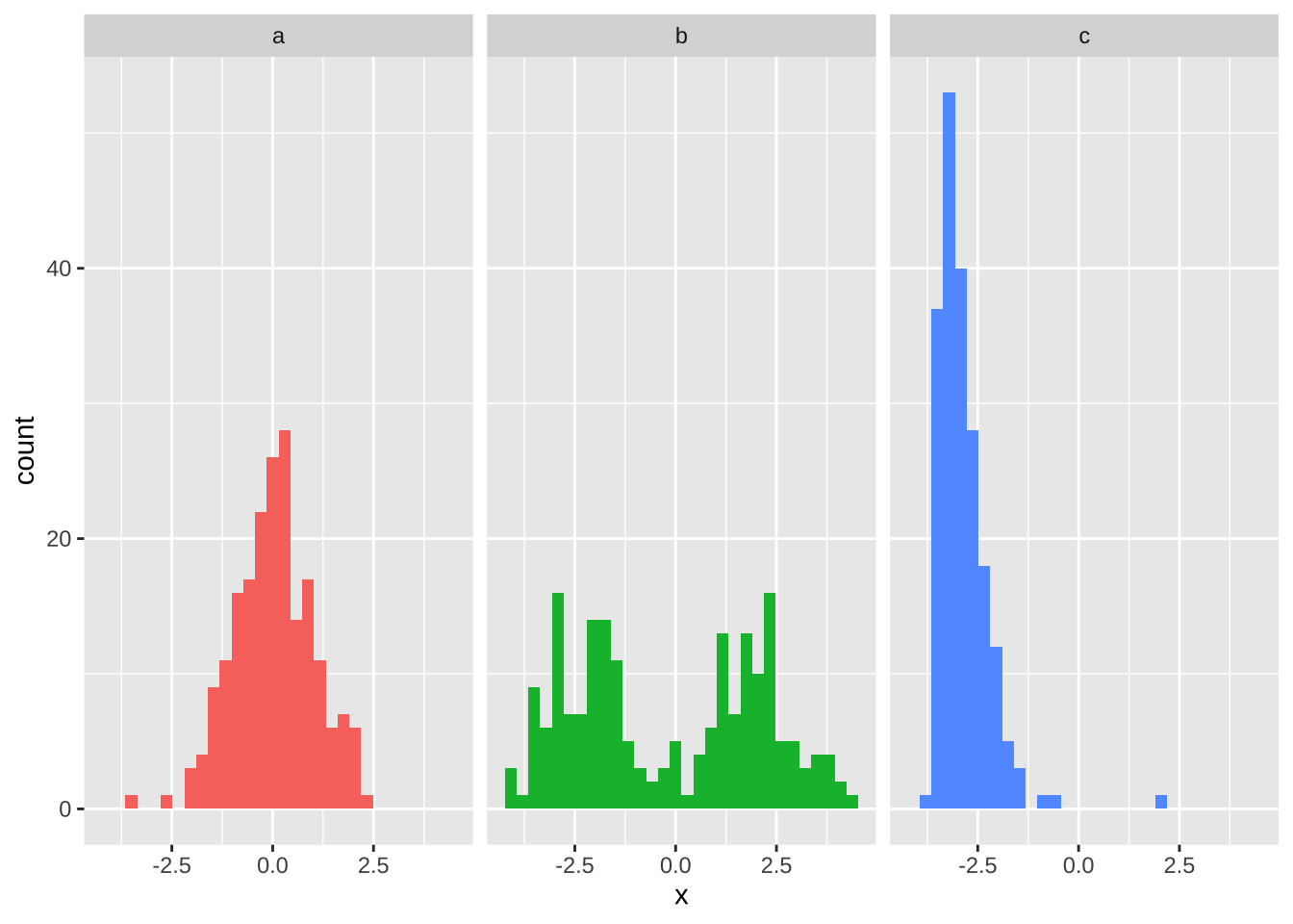
Why does the shape of a distribution change the meaningfulness of some summary stats like the mean and standard deviation. Take for example the three plots below
Why are barplots +/- standard errors are not a good way to display continuous variables?
Which of the questions above would you like to focus on most in class?
What stats concept trips you up?
What R trips you up?