Chapter 11 Uncertainty
These notes accompany portions of Chapter 4 — Estimating with Uncertainty — which we first encountered in Section 7, and the “Bootstrap Standard Errors and Confidence Intervals” section of Chapter 19 (pages 647-654) of our textbook. The reading below is required, Whitlock and Schluter (2020) is not.
If you want a different (or another) presentiation of this material, I highly recommend Chapter 8 of Ismay and Kim (2019) as an optional reading.
If you want to read more about visualizing uncertainty, I suggest Clause Wilke’s chapter on the subject (Wilke 2019).Motivating scenarios: You have a sample and made an estimate, and want to communicate the precision of this estimate.
Learning goals: By the end of this chapter you should be able to:
- Explain why the idea of the sampling distribution is useful in communicating our uncertainty in an estimate.
- Describe the challenge we have in building a sampling distribution from a single sample.
- Explain how we can build estimate a sampling distribution from a single sample by resampling with replacement.
- Use R to bootstrap real data.
- Describe the concept of the confidence interval.
- Calculate bootstrapped standard errors and bootstrapped confidence intervals.
- Recognize why/when we would (or would not) use the bootstrap to quantify uncertainty.
- Know how to visualize uncertainty in R.
In addition to this reading, the other assignments are:
- Take a single bootstrap (described below)
- Watch from 0:54 to 3:32, plus 4:53 to 6:49, and 10:50-12:20 from this Crash Course Statistics video about confidence intervals (split into three below).
- Explore the webapp about confidence intervals, below.
- Complete the uncertainty quiz below and finish on canvas.
11.1 Review of relevant material:
In Section 10 we sampled from a population many times to build a sampling distribution. But, if we had data for an entire population, we would know population parameters, so there would be no reason to calculate estimates from a sample.
In the real world we have a small number (usually one) of sample(s) and we want to learn about the population. This is a major a major challenge of statistics (See Section 1).
11.1.1 Review: Populations have parameters
We conceptualize populations as truth with true parameters out there.
11.1.2 Review: Sampling involves chance
Because (a good) sample is taken from a population at random, a sample estimate is influenced by chance.
11.1.3 Review: The standard error
The sampling distribution – a histogram of sample estimates we would get by repeatedly sampling from a population – allows us to think about the chance deviation between a sample estimate and population parameter induced by sampling error.
The standard error quantifies this variability as the standard deviation of the sampling distribution.
Reflect on the two paragraphs above. They contain stats words and concepts that are the foundation of what we are doing here.
- Would this have made sense to you before the term?
- Does it make sense now? If not, take a moment, talk to a friend, email Yaniv or Anna, whatever you need. This is important stuff and should not be glossed over.
11.2 Estimation with uncertainty
Because estimates from samples take their values by chance, it is irresponsible and misleading to present an estimate without describing our uncertainty in it, by reporting the standard error or other measures of uncertainty.
11.2.1 Generating a sampling distribution
Question: We usually have one sample, not a population, so how do we generate a sampling distribution?
Answer: With our imagination!!! (Figure 11.1).
What tools can our imagination access?
- We can use math tricks that allow us to connect the variability in our sample to the uncertainty in our estimate.
- We can simulate the process that we think generated our data.
- We can resample from our sample by bootstrapping (describe below).

Figure 11.1: We use our imagination to build a sampling distribution by math, simulation, or bootstrapping.
Don’t worry about the first two too much – we revisit them throughout the course. For now, just know that whenever you see this, we are imagining an appropriate sampling distribution. Here we focus on bootstrapping.
11.2.1.1 Resampling from our sample (Bootstrapping)
While statistics offers no magic pill for quantitative scientific investigations, the bootstrap is the best statistical pain reliever ever produced.As quoted in Cochran (2019)
So we only have one sample but we need to imagine resampling from a population. One approach to build a sampling distribution in this situation is to assume that your sample is a reasonable stand-in for the population and resample from it.
Of course, if you just put all your observed values down and picked them back up, you would get the same estimate as before. So we resample with replacement and make an estimate from this resample – that is, we
- Pick an observation from your sample at random.
- Note its value.
- Put it back in the pool.
- Go back to (1) until you have as many resampled observations as initial observations.
- Calculate an estimate from this collection of observations.
- After completing this you have one bootstrap replicate.
Assignment: Physically generate a bootstrap replicate. We will soon learn how to conduct a bootstrap in R, but I find that getting physical helps it all be real, and gives us more appreciation for what is going on in a bootstrap. So, our assignment is to generate a single bootstrap replicate by brute force
- Find a sample of about twenty of something that is easy to quantify, I suggest the date on n = twenty pennies if you have them. If all else fails you can write down values on a piece of paper (e.g. the point differential for Timberwolves games this season, the length of twenty songs on your itunes etc..)
- Estimate the sample mean (i.e. What is the mean date of issue of pennies in your sample).
- Shove your observations in a bag or sock or something.
- Generate an estimate from a single bootstrap replicate. Sample n observations with replacement, and calculate your estimate from this bootstrap replicate.
- On canvas, you will need to state what you resampled, what population it was meant to represent. If it is or is not a random sample of that population (with some explanation about why), the value of the sample estimate, the value of the bootstrapped estimate, and how/why they differed. Reflect on what is going on here.
While the exercise above was useful, it would be tedious and unfeasible to do this more than a handful of times. Luckily, we don’t have to, we can use a computer to conduct a bootstrap.
Bootstrapping computation and example: Fireflies!

Figure 11.2: Firefly pulsing.
EXAMPLE Say we are studying the duration of light pulses of male fireflies, Photinus ignitis, a species in which females prefer to mate with males that are bright for longer pulses. We can look at pulse duration data, collected by Cratsley and Lewis (2003) data, to estimate the mean duration of pulses and the uncertainty in this estimate.
firefly_file <- "https://whitlockschluter3e.zoology.ubc.ca/Data/chapter04/chap04q07FireflyFlash.csv"  ### link to data
firefly     <- read_csv(firefly_file) %>% # load data
  mutate(id = 1:n(),
         id = factor(id))   # add an id (for shits  -- this isnt necessary]
First (as always) let’s look at the actual data. You could do this with glimpse(), view(), or just typing firefly.
Calculating estimates from the data
Now we make an estimate from the data! We can bootstrap any estimate - a mean, a standard deviation, a median, a correlation, an F statistic, a phylogeny, whatever. But we will start with a mean for simplicity.
sample_estimate <-  firefly  %>%
  summarise(mean_flash = mean(flash)) %>%### Summarize the data (let's summarize the mean )
  pull()

round(sample_estimate , digits = 2)
## [1] 95.94So, our sample estimate is that the mean firefly pulse rate is 95.94. But that is just our sample.
Now we cannot learn the true population parameter, but we can bootstrap to get a sense of how far from the true parameter we expect an estimate to lie.
Resampling our data (with replacement) to generate a single bootstrap replicate
First, let’s use the slice_sample() function to generate a sample of the same size. You will notice that this code is very similar to what we wrote for sampling (Section 10.2) except that we
- Sample with replacement – that is, we tell R to toss each observation back and mix up the bag every time, outlined in above.
- Take a (resampled) sample that is the same size as our sample, rather than a subsample of our population.
# One bootstrap replicate
resampled_fireflies <- firefly  %>%
  slice_sample(prop = 1, replace = TRUE) # resample the data with replacement
So, lets look at the resampled data:
To confirm that my resampling with replacement worked, let’s make sure some we see some individuals more than once, and some not at all.
resampled_fireflies                %>%
  group_by(id, .drop=FALSE)        %>%   # .drop = FALSE on this factor means that we keep count for individuals with zero, instead of losing them
  tally(sort = TRUE)               %>%   # count how many times we see each individual in the resample, and arrange from most to fewest times.
  mutate(id = fct_reorder(id, n,.desc = TRUE)) %>%  # tell R we want to list numbers in the order of number of observations, not from 1 to n
  ggplot(aes(x=id, y = n))+ # set up the ggplot
  geom_col()              + # make a bar plot
  labs(title = "Distribution of resampled individuals in our bootstrap")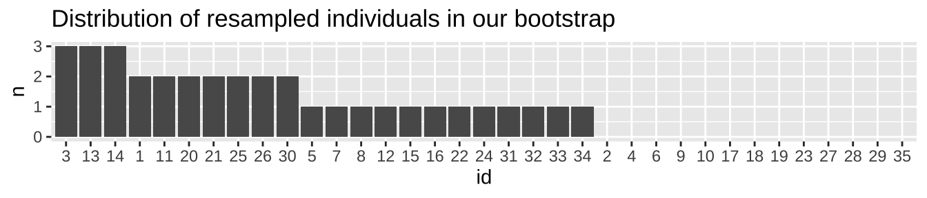
So, now that it looks like we resampled with replacement correctly (we see some individuals a few times, some zero times), let’s make an estimate from this resampled data.
resampled_fireflies  %>%
  summarise(mean_flash = mean(flash)) ### Summarize the data (lets summarize the mean)
## # A tibble: 1 × 1
## mean_flash
## <dbl>
## 1 94.6So, the difference between the sample estimate and the resample-based estimate is 1.37. But this is just one bootstrap replicate.
Resampling many times to generate a bootstrap distribution
Let’s do this many (10,000) times with the replicate() function, much like we did Section 10.3.1.1 – except we set prop = 1 and replace = TRUE (rather than size = sample.size - were is sample.size\(<\) population.size, and replace = FALSE). We then visualize this bootstrapped sampling distribution as a histogram.
n.reps <- 10000

firefly_boot <- replicate(n = n.reps, simplify = FALSE, # tell R to do this a bunch, and to keep each result as its own tibble
    expr = slice_sample(firefly, prop =  1, replace = TRUE) %>%    # same code as above
    summarise(boot_mean_flash = mean(flash)))        %>%           # calculate proportion with mean()
  bind_rows()

# recall we're grouped by replicate when we come out of rep_sample_n()

boot_dist_plot <- ggplot(firefly_boot, aes(x = boot_mean_flash)) +   # assign plot to a variable
  geom_histogram(fill = "firebrick", color = "white", bins=40)+
  geom_vline(xintercept = sample_estimate, lty = 2)+ # add a line to show the sample estimate
  labs(title = "The bootstrapped sampling\ndistribution",
       subtitle = "Firefly pulse time (n = 35).")

boot_dist_plot  ## show the plot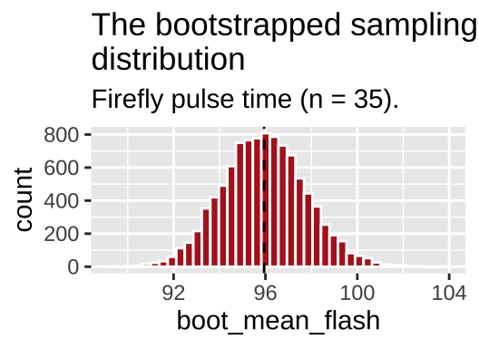
Figure 11.3: The bootstrapped sampling distribution. Dashed line represents sample estimate.
AWESOME! So what happened here? We had a sample, not a population. but we resampled from it with replacement to generate a sampling distribution. This histogram depicts the expected sampling error from a population that resampled our sample. So we can use this to get a sense of the expected sampling error in our actual population which we do not explore beyond this sample.
Note that this is a good guide - but is not foolproof. Because we start with a sample from the population, this bootstrapped sampling distribution, will differ from our population sampling distribution – but it is a reasonable estimate!!!
Bootstrapping: Notes and considerations
The bootstrap is incredibly versatile - it can be used for any estimate, and, with enough care for study design, can be applied to almost any statistical problem. Because the bootstrap does not assume much about the shape of the variability in a population, it can be used when many other method we cover this term fail.
Because it requires some computer skills, and because it solves hard problems, the bootstrap is often taught at the end of an intro stats course. For example, the bootstrap is covered in Computer intensive methods of our textbook (Section 19.2 of Whitlock and Schluter (2020)). But I introduce it early because it is both useful and helps us think about the sample standard error and confidence intervals (below).
If you don’t know anything about statistics, learn the bootstrap. Seriously, think of it as a “statistical pain reliever”!! My new favorite term for the approach that underlies almost everything I do... https://t.co/jCHozq80oM
— Ryan Hernandez (@rdhernand) March 9, 2019
That said, a bootstrap is not always the best answer.
Bootstrapping requires a reasonable sample size, such that the breadth of values in the population is sampled [as a thought experiment, imagine bootsrapping with one or two observations – the answer would clearly be nonsense]. The minimum sample size needed depends on details of the population distribution etc.., but in many cases a sample of size twenty is large enough for bootstrapping to be reasonable.
Because a bootstrap depends on chance sampling, it will give (very slightly) different answers each time. This can be frustrating.
11.2.2 Estimating the standard error
In Section 10 we learned how to generate a (potentially infinite) number of samples of some size from a population to calculate the true standard error. But, in the real world we estimate the standard error from a single sample.
Again, we can use our imagination to calculate the standard error, and again we have math, simulation, and resampling as our tools.
11.2.2.1 The bootstrap standard error
Here, we focus on the bootstrap standard error as an estimate of the standard error. Because the standard error measures the expected variability among samples from a population as the standard deviation of the sampling distribution, the bootstrap standard error estimates the standard error as the standard deviation of the bootstrapped distribution.
We already did the hard work of bootstrapping, so now we find the bootstrap standard error as the standard deviation of the bootstrapped sampling distribution 11.3.
firefly_boot_SE <- firefly_boot %>%
  summarise(SE = sd(boot_mean_flash))

firefly_boot_SE
## # A tibble: 1 × 1
## SE
## <dbl>
## 1 1.81What is the difference between the bootstrapstandard error described here and and standard error in Section 10?
In Section 10 we (1) took many samples from our population, (2) summarized them to find the sampling distribution, and (3) took the standard deviation of these estimates to find the population standard error.
In bootstrapping, we (1) resample our sample many times, (2) summarize these resamples to approximate (a.k.a. fake) a sampling distribution, and (3) take the standard deviation of these estimates to estimate the standard error as the bootstrap standard error.
11.2.3 Confidence intervals
Watch the videos below for a nice explanation of confidence intervals. Note: I split this video into three parts and excluded the bits about calculating confidence internals under different scenarios because that’s a distraction at this point. We will return to calculations as they arise, but for now we will estimate confidence intervals by bootstrapping.
part 1
Figure 11.4: Explanation of confidence intervals from Crash Course Statistics. I split this into three parts removing the bits that arent immediately relevant to us.
part 2
part 3
As explained in the videos above, Confidence intervals provide another way we describe uncertainty. To do so we agree on some level of confidence to report, with 95% confidence as a common convention.
Confidence intervals are a bit tricky to think and talk about. I think about a confidence interval as a net that does or does not catch the true population parameter. If we set a 95% confidence level, we expect ninety five of every one hundred 95% confidence intervals to capture the true population parameter.
Explore the webapp from Whitlock and Schluter (2020) to make this idea of a confidence interval more concrete. Try changing the sample size (\(n\)), population mean (\(\mu\)), and population standard deviation (\(\sigma\)), to see how these variables change our expected confidence intervals.
Figure 11.5: Webapp from Whitlock and Schluter (2020) showing the disrtibution of confidence interavals. Find it on their website.
Because each confidence interval does or does not capture the true population parameter, it is wrong to say that a given confidence interval has a given chance of catching the parameter. The parameter is fixed, it is the chance sampling of the sample from which we calculate the confidence interval where the chance happens.
So, how do we calculate confidence intervals? Like the standard error, we can calculate confidence intervals with math, simulation or resampling. We explore the other options in future Sections, but discuss the bootstrap based confidence interval here.
11.2.4 The bootstrap confidence interval
We can estimate a specified confidence interval as the middle region consisting of that proportion of bootstrap replicates. So the edges between the middle 95% of bootstrap replicates and more extreme resamples denote the 95% confidence interval. We can use the quantile() function in R to find these breaks of the bootstrap.
firefly_boot_CI <- firefly_boot %>%
  summarise(CI         = c("lower 95", 'upper 95'), # add a column to note which CIs we're calcualting
            mean_flash = quantile(boot_mean_flash ,probs = c(.025,.975)))  # boundaries separating the middle 95% from the rest of our bootstrap replicates.

firefly_boot_CI
## # A tibble: 2 × 2
## CI mean_flash
## <chr> <dbl>
## 1 lower 95 92.5
## 2 upper 95 99.6So we are 95% confident that the true mean is between 92.49 and 99.57.
A confidence interval should be taken as a guide, not a bright line. There is nothing that magically makes 99.47 a plausible value for the mean and 99.67 implausible.
We can add these confidence intervals to our plot with geom_vline()
boot_dist_plot  +
  geom_vline(xintercept = pull(firefly_boot_CI, mean_flash),
             color      = "blue")+
  annotate(x = 102, y = 650, color = "blue",
           geom = "text", label = "95% CI", lty = 3)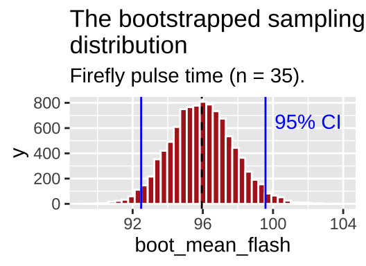
Figure 11.6: The bootstrapped sampling distribution. Dashed black line represents sample estimate. Dotted blue line shows 95% confidence limits.
11.3 Visualizing uncertainty
In addition to stating our uncertainty in words, we should show our uncertainty in plots. The most common display of uncertainty in a plot is the 95% confidence interval, but be careful, and clear, because some people report standard error bars instead of confidence intervals (and others display measures of variability rather than uncertainty).
The code below shows how we 95% confidence intervals to out ggplot by telling the stat_summary() function that we want R to calculate and show bootstrap based 95% confidence limits.
ggplot(firefly, aes(x = "Duration", y = flash))+
  geom_jitter(width = .1, color = "firebrick", alpha = .6, size = 3)+
  stat_summary(fun.data = mean_cl_boot,
position = position_nudge(x = .2, y = 0)) # move line over some so as to not hide our data. 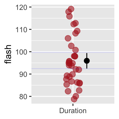
Figure 11.7: R will calculate and display 95% bootstrap confidence limits if we add stat_summary(fun.data =mean_cl_boot). Faint blue horizontal lines (from my boostrap, above), closely match the bootsrap R just did.
stat_summary() uses the Hmisc package, so if this code is not working for you, type install.packages("Hmisc").
While this display is most traditional Clause Wilke has recently developed a bunch of fun new approaches to visualize uncertainty (see his R package, ungeviz), and the chapter on the subject (Wilke 2019), is very fun. We show one such sample in Figure 11.8.
Figure 11.8: A novel form of visualizing uncertainty provides a smoother view of uncertainty, to complement the traditional confidence limits based display.
11.4 Common mathematical rules of thumb
So long as a sample isn’t too small, the bootstrap standard error and bootstrap confidence intervals are reasonable descriptions of uncertainty in our estimates.
Above, we also pointed to mathematical summaries of uncertainty. Throughout the term, we will cover different formulas for the standard error and 95% confidence interval, which depends on aspects of the data – but rough rules of thumb are:
- For normally distributed data the standard error (aka the standard deviation of the sampling distribution) equals the standard deviation divided by the square root of the sample size, so we often approximate the sample standard error as \(SE_x = \frac{s_x}{\sqrt{n}}\).
- The 95% confidence interval is approximately the mean plus or minus two times the standard error.
11.5 Uncertainty Quiz
11.5.1 Optional: Use existing R packages to bootstrap for you
There are many R packages that have functions to perform a bootstrap. I like to have us write the bootstrap ourselves because I think it clarifies what is really happening, and because its sometimes easier towrite your own code than figure out a package.
Here, I show two commonly used packages – called infer and [mosaic](https://github.com/ProjectMOSAIC/mosaic). Both packages do way more than bootstrapping, and have been developed in concert with statistics courses.
11.5.1.1 The infer package
Check out details here
boot_firefly_mean_flash <-  firefly %>%
    specify(response = flash) %>%
    generate(reps = 10000, type = "bootstrap") %>%
    calculate(stat = "mean")

boot_firefly_mean_flash %>%
  summarise(CI         = c("lower 95", 'upper 95'), # add a column to note which CIs we're calcualting
            mean_flash = quantile(stat ,probs = c(.025,.975)))
## # A tibble: 2 × 2
## CI mean_flash
## <chr> <dbl>
## 1 lower 95 92.4
## 2 upper 95 99.711.5.1.2 The mosiac package
Check out details here
library(mosaic)## Registered S3 method overwritten by 'mosaic':
## method from
## fortify.SpatialPolygonsDataFrame ggplot2##
## The 'mosaic' package masks several functions from core packages in order to add
## additional features. The original behavior of these functions should not be affected by this.##
## Attaching package: 'mosaic'## The following object is masked from 'package:Matrix':
##
## mean## The following object is masked from 'package:plotly':
##
## do## The following objects are masked from 'package:car':
##
## deltaMethod, logit## The following objects are masked from 'package:infer':
##
## prop_test, t_test## The following object is masked from 'package:ggthemes':
##
## theme_map## The following object is masked from 'package:cowplot':
##
## theme_map## The following objects are masked from 'package:dplyr':
##
## count, do, tally## The following object is masked from 'package:purrr':
##
## cross## The following object is masked from 'package:ggplot2':
##
## stat## The following objects are masked from 'package:stats':
##
## binom.test, cor, cor.test, cov, fivenum, IQR, median, prop.test,
## quantile, sd, t.test, var## The following objects are masked from 'package:base':
##
## max, mean, min, prod, range, sample, sum# bootstrap
boot_firefly_mean_flash <- mosaic::do(10000) * mean( ~ flash, data = resample(firefly))
# find conf interval
confint(boot_firefly_mean_flash, level = 0.95, method = "quantile")## name lower upper level method estimate
## 1 mean 92.4 99.57143 0.95 percentile 95.94286detach("package:mosaic", unload=TRUE)
#detach("package:infer", unload=TRUE)As you see this matches our own coding