Chapter 9 Review of R and New tricks
By now, we have hopefully gotten the hang of getting things done in R. But we’re all in a different place. Some of us still have some fundamental things we don’t understand. Others feel ok on the whole, but there might be something that you don’t quite get, or a bunch of confusing errors that you haven’t understood.
Maybe you have R questions related to work you have done outside of his class, or you are curious about base R.
Or you want to make nice reproducible reports in RMarkdown and/or learn how to organize an RProject, or organize make a collaborative open project on github.
This lesson is designed to give you a chance to catch up on R, connect the dots between what you have learned, review, and/or learn new things. This should help you prepare for your first major assignment of an exploratory data analysis, due on Monday.
9.1 When R goes wrong
R can be fun, useful and empowering, but it can also be a bummer. Sometimes it seems like you’ve done everything right, but things still aren’t working. Other times, you just can’t figure out how to do what you want. When this happens it is natural to tense up, curse, throw $h!t etc… While some frustration is OK, you should try to avoid sulking. Here’s what I do.
- Take a deep breath.
- Copy and paste and try again. If that doesn’t work, go to 3.
- Look at the code for any common issues (like those in Section 9.1.2, below). If I see one of these issues, I fix it and feel like a champ. If not, I go to step 4.
- Remember that google is my friend, use it. I usually copy the error message R gives and paste it into google. Does this give me a path towards solving this? If so give it a shot, if not, go to 5.
- Take a walk around the house, grab a drink of water, get away from the computer for a minute. Then think about what I was trying to do and return to the computer to see if I’ve done it right and if that time away allowed me to see mistakes I missed before. If I see the issue, I fix it and feel like a champ. If not, I go to step 6.
- Move on, do something else and come back to it later (7). If you have more R to work on, try that (unless you need a break). If you’re not going to do more R, you should probably close your RStudio session.
- OK back to it. Reopen RStudio and work through your code. Do you see the issue now? If so fix it, if not move onto 8.
- Explain the issue to a friend / peer. I often figure out what I did wrong, when I explain it. Like “I said add 5+5 and it kept giving me 10, when the answer should have been 25.” And then I realize I added when I wanted to multiply. Or maybe your friend figures it out.
- How important is this thing? Can I do something slightly different that is good enough? If so I try that. If it’s essential,
- Find an expert or stackoverflow or something.
Troubleshooting lessons I guess I'll just relearn forever:
— Allison Horst (@allison_horst) January 4, 2020
- take a break
- it's almost certainly not a bug
- extra eyes are awesome
- spelling pic.twitter.com/J17S8I6b3W
9.1.0.1 Run only a few lines
When you type more complex stuff errors are bound to show up somewhere. I suggest running each line one at a time (or at least running a few lines at a time to unstick yourself if you found an error 9.1).
include_graphics("images/run a few lines.jpeg")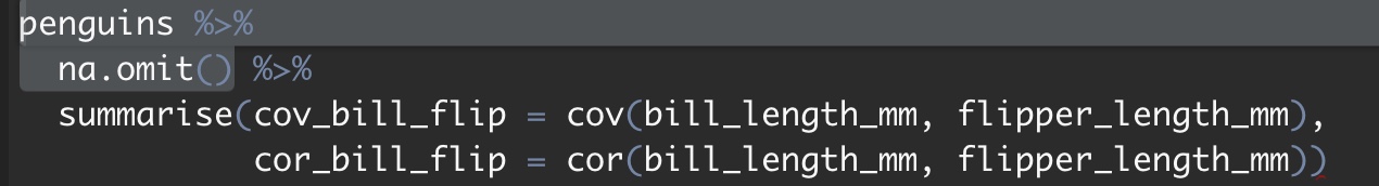
Figure 9.1: You can run a few lines by highlighting what you want to turn (make sure not to end on a pipe %>%).
9.1.1 Warnings and Errors, Mistakes and Impasses
Before digging into the common R errors, lets go over the four ways R can go wrong.
A warning. We did something that got
Rnervous, and it gives us a brief message. It is possible everything is ok, but just have a look. I think of this as a yellow light. The most common warning I get is the harmlesssummarise() ungrouping output (override with .groups argument).An error. We did something that R does not understand or cannot do. R will stop working and make us fix this. I think of this as a red light.
A mistake. Our communication with R broke down – it thought we were doing one thing but we wanted it to do another. Mistakes are the most likely to cause a big problem. So, remember that just because R works without an error or warning, does not mean it did what we hoped.
An impasse. There’s something we want to do, but can’t figure it out.
Be mindful of these types of issues with R as you code and as you read the common errors below.
9.1.2 Common gotcha’s
I share my most common mistakes, below. I note that these are my common mistakes. If you find that you often make different sorts of mistakes, email me with them, and I’ll add them.
9.1.2.1 Spelling / capitilization etc
R cant read your mind (although tab-completion in RStudio is awesome), and pays attention to capital letters. Spellng errors are my most common mistake. For example, the column, Sepal.Length, in the iris dataset has sepal lengths for a bunch of individuals. Trying to select the column by typing any one of the options below will yield a similar error:
dplyr::select(iris, sepal.length)
dplyr::select(iris, Sepal_Length)
dplyr::select(iris, Sepal.Lngth)
## Error in `dplyr::select()`:
## ! Can't subset columns that don't exist.
## ✖ Column `Sepal.Lngth` doesn't exist.Similarly, you might misspell the function:
dplyr::selct(iris, Sepal.Length)## Error: 'selct' is not an exported object from 'namespace:dplyr'So, check for these mistakes and fix the code above to look like this:
dplyr::select(iris, Sepal.Length)## # A tibble: 6 × 1
## Sepal.Length
## <dbl>
## 1 5.1
## 2 4.9
## 3 4.7
## 4 4.6
## 5 5
## 6 5.49.1.2.2 Confusing == and =
Consecutive equals signs == ask if the thing on the right equals the thing on the left. For example, if I want to know if two equals six divided by two, I type 2 == (6/2) and R says FALSE. But what if I accidentally type (6/2) = 3. In this case R gets very confused.
2 = (6/2)## Error in 2 = (6/2): invalid (do_set) left-hand side to assignmentThis confusion arises because we told R to make two equal six divided by two, which is nonsense.
two <- 2But it could be worse than nonsense. Say the value two is assigned to two, and now we ask if two equals (6/2). Asking with a ==, as in two == (6/2), gives us our expected answer: FALSE. But typing two = 6/2 does not ask if two equals 6/2, rather it tells R that two equals 6/2 for now, returning unexpected results like that below.
two^2## [1] 9This is one of many cases in which R does what we say and does not warn of an error, but does not do what we hoped it would.
One more note while we’re here: The clarity and utility of R’s error messages vary tremendously.
For example, if we confuse = and == inside the filter() function in the dplyr package, R gives a very useful error message. For example, say we mess up in asking R to only return data for Iris setosa from the iris data set.
filter(.data = iris, Species = "setosa")## Error in `filter()`:
## ! We detected a named input.
## ℹ This usually means that you've used `=` instead of `==`.
## ℹ Did you mean `Species == "setosa"`?By contrast doing a similar operation in base R (which you may have seen previously, but we don’t cover in this course) , yields a less clear error message:
iris[ iris$Species = "setosa", ]## Error: <text>:1:20: unexpected '='
## 1: iris[ iris$Species =
## ^9.1.2.3 Confusing = and <-
As we’ve seen throughout the course, we use the global operator, to assign values to variables. But inside a function we use the = sign to assign values to argument in a function. Using the global operator in a function does a bunch of bad things.
Say we wanted to sample a letter from the alphabet at random. Typing sample(x = letters, size =1), will do the trick and will not assign any value to x outside of that function.
#### DO THIS
sample(x = letters[1:10], size =1)
## [1] "b"x## Error in eval(expr, envir, enclos): object 'x' not foundThe error above is a good thing – we wanted to sample letters, not have x equal the letters. By contrast, using <- to assign values to arguments has bad consequences.
#### DONT DO THIS
sample(x <- letters, size =1)
## [1] "y"x## [1] "a" "b" "c" "d" "e" "f" "g" "h" "i" "j" "k" "l" "m" "n" "o" "p" "q" "r" "s"
## [20] "t" "u" "v" "w" "x" "y" "z"This is BAD. We did not want to assign the alphabet to x, we just wanted the sample() function to sample from the alphabet. Bottom line:
- Use the
=sign to assign values to arguments in a function.
- Use
<-to assign values to variables outside of a function.
- Use
==to ask if one thing equals another.
9.1.2.4 Dealing with missing data
Often our data includes missing values. When we do math on a vector including missing values, R will return NA unless we tell it to do something else. See below for an example:
my_vector <- c(3,1,NA)
mean(my_vector)
## [1] NADepending on the function, we have different ways of telling R what to do with missing data. In the mean() function, we type.
mean(my_vector, na.rm = TRUE)## [1] 2We have to be extra careful of missing values when doing math ourselves. If we found the mean of my_vector by dividing its sum by its length, like this: sum(my_vector) / length(my_vector) = NA, we would have the wrong answer. So be careful and avoid this mistake.
9.1.2.5 Conflicts in function names
Each function in a package must be unique. But functions in different packages can have the same name and do different things. This means we might be using a totally different function than we think. If we’re lucky this results in an error, and we can fix it. If we’re unlucky, this results in a bad mistake.
We can avoid this mistake by typing the package name and two colons and then the function name (e.g. dplyr::filter) before using any function. But this is quite tedious. Installing and loading the conflicted package, which tells us when we use a function that is used by more than one package loaded, resulting in a warning that we can fix!
9.1.2.6 Mistakes in assignment
I often mess up in assigning values to variables. I do so in a few different ways, I:
- Forget to assign a variable to memory,
- I use the variable before it’s assigned,
- I don’t update my assignment after doing something, or
- I overwrite my old assignment.
I’ll show you what I mean and how to spot and fix these common issues…
9.1.2.6.1 Mistakes in assignment: Not in memory
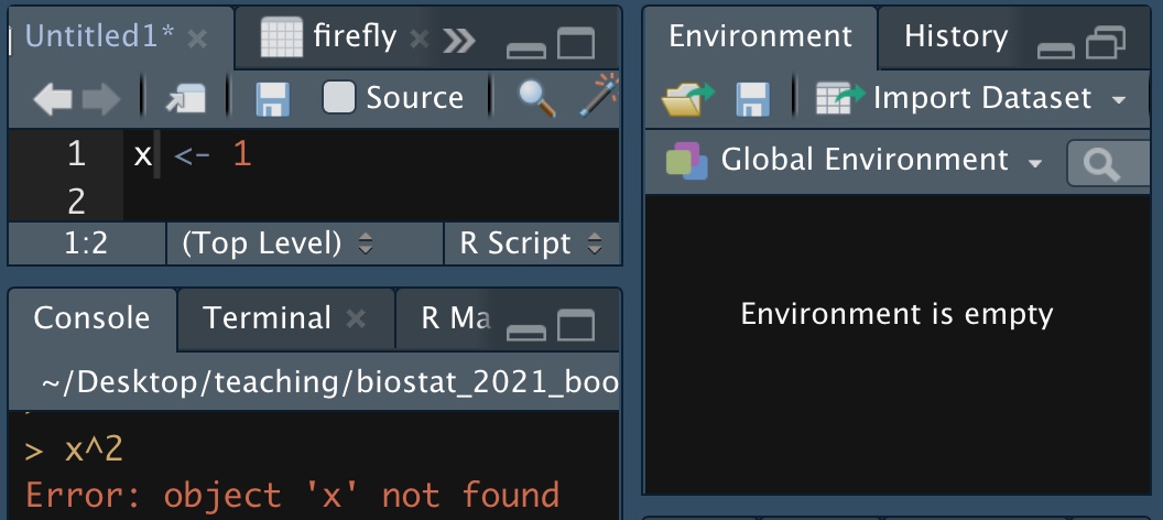
Figure 9.2: I did not assign the value one to x.
As the example in Figure 9.2 shows, typing a value into an R script is not enough. We need to enter it into memory. You can do this by either, hitting ctrl + shift, or /command + shift, or hitting the run button in the RStudio IDE, or copying and pasting into the terminal widow.
To see all the variables in Rs memory, check the environment tab in the RStudio IDE, or use the ls() function with no arguments.
9.1.2.6.2 Mistakes in assignment: Wrong order
If you want to square x, (as in Figure 9.2), you must assign it a value first. This mistake is quite similar to the one above.
x^2
x  <-  1
## Error in x^2: non-numeric argument to binary operator9.1.2.6.3 Mistakes in assignment: Not updating assignment
Another common mistake is to run some code but not assign the output to anything. So, for example we wanted to make a density plot of the ratio of petal width to sepal width. Can you spot the error in the code below?
iris %>%
  mutate(petal_to_sepal_width = Petal.Width / Sepal.Width)
## # A tibble: 150 × 6
## Sepal.Length Sepal.Width Petal.Length Petal.Width Species petal_to_sepal_wid…
## <dbl> <dbl> <dbl> <dbl> <fct> <dbl>
## 1 5.1 3.5 1.4 0.2 setosa 0.0571
## 2 4.9 3 1.4 0.2 setosa 0.0667
## 3 4.7 3.2 1.3 0.2 setosa 0.0625
## 4 4.6 3.1 1.5 0.2 setosa 0.0645
## 5 5 3.6 1.4 0.2 setosa 0.0556
## 6 5.4 3.9 1.7 0.4 setosa 0.103
## 7 4.6 3.4 1.4 0.3 setosa 0.0882
## 8 5 3.4 1.5 0.2 setosa 0.0588
## 9 4.4 2.9 1.4 0.2 setosa 0.0690
## 10 4.9 3.1 1.5 0.1 setosa 0.0323
## # … with 140 more rowsggplot(iris, aes(x = petal_to_sepal_width, fill = Species )) +
geom_density(alpha = .5)## Error in FUN(X[[i]], ...): object 'petal_to_sepal_width' not found
We clearly calculated petal_to_sepal_width, above, so why can’t R find it? The answer is that we did not save the results. Let’s fix this by assigning our new modifications to iris.
iris <- iris %>%
mutate(petal_to_sepal_width = Petal.Width / Sepal.Width)
ggplot(iris, aes(x = petal_to_sepal_width, fill = Species )) +
  geom_density(alpha = .5)
9.1.2.6.4 Mistakes in assignment: Overwriting assignments
Above, I showed how failing to reassign after doing some calculation can get us in trouble. But other times, reassigning can cause it own problems.
For example, let’s say I want to calculate mean() petal to sepal widths for each species and then make the same plot as above.
iris <- iris        %>%
  group_by(Species) %>%
  dplyr::summarize(mean_petal_to_sepal_width = mean(petal_to_sepal_width))

ggplot(iris, aes(x = petal_to_sepal_width, fill = Species )) +
  geom_density(alpha = .5)
## Error in FUN(X[[i]], ...): object 'petal_to_sepal_width' not found
So, what went wrong here? Let’s take a look at what I did to iris:
iris## # A tibble: 3 × 2
## Species mean_petal_to_sepal_width
## <fct> <dbl>
## 1 setosa 0.0719
## 2 versicolor 0.480
## 3 virginica 0.684Ooops, we just have species means. By combining summarise with a reassignment, we replaced the whole iris dataset with a summary of means. In this case, it’s better to assign your output to a new variable…
iris_petal2sepalw_bysp <- iris        %>%
  group_by(Species) %>%
  dplyr::summarize(mean_petal_to_sepal_width = mean(petal_to_sepal_width), .groups= "drop_last")

ggplot(iris, aes(x = petal_to_sepal_width, fill = Species )) +
  geom_density(alpha = .5)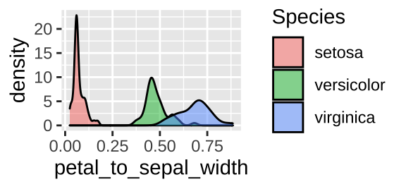
No worries though if you have your code well laid out, you can just rerun everything until the pint before you made this mistake and you’re back in business.
So when should we reassign to the old variable name, and when should we assign to a new name? My rule of thumb is to reassign to the same variable when I add things to a tibble, but do not change existing data, while I assign to a new variable when values change or are removed (with some exceptions).
But what if you wanted the mean in the same tibble as the initial data so you could add lines for species means? You can so this with mutate() instead of summarise().
iris <- iris        %>%
  group_by(Species) %>%
  dplyr::mutate(mean_petal_to_sepal_width = mean(petal_to_sepal_width), .groups= "drop_last")

ggplot(iris, aes(x = petal_to_sepal_width, fill = Species)) +
  geom_density(alpha = .5)+
  geom_vline(aes(xintercept = mean_petal_to_sepal_width, color = Species), lty = 2)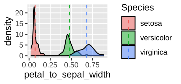
9.1.2.7 Just because you didn’t get an error doesn’t mean R is doing what you want (or think):
Say you want to reassign x to the value 10, and you want y to equal x$^2$ (so y should be 100). The code below messes this up by assigning the value x^2 to y before it setting x to 10. This means that y is using the older value x, which equals 1, set above.
y  <-   x^2
x  <-   10
print(y)
## [1] 19.1.2.8 Unbalanced parentheses, quotes, etc…
Some things, like parentheses and quotes come in pairs. Too many or too few will cause trouble.
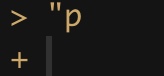
If you have one quote or parenthesis open, without its partner (e.g.
"p), R will wait for you to close it. With a short piece of code you can usually figure out where to place the partner. If the code is long and it’s not easy to spot, hitescapeto start that line of code over.Also, in a script, clicking the space after a parenthesis should highlight its partner and bring up a little X in the sidebar to flag missing parentheses.
Unbalanced parentheses cause R to report an error (below).
c((1)## Error: <text>:2:0: unexpected end of input
## 1: c((1)
## ^9.1.2.9 Common issues in ggplot
9.1.2.9.1 Using %>% instead of +
We see that tidyverse has two ways to take what it has and keep moving.
When dealing with data, we pipe opperations forward with the
%>%operator. For example, we toldRto tak our tibble and then pull out our desired coumn, abovename_of_tibble %>% pull(var = name_of_column).When building a plot, we add elements to it with the
+sign. For example, in a scatterplot, we type:ggplot(data = <name_of_tibble>, aes(x=x_var, y = y_var)) + geom_point().
I occasionally confuse these and get errors like this:
ggplot(iris, aes(x = Petal.Length, y = Petal.Width)) %>%
  geom_point()
## Error in `validate_mapping()`:
## ! `mapping` must be created by `aes()`
## Did you use %>% instead of +?Or
iris +
  summarise(mean_petal_length = mean(Petal.Length))
## Error in mean(Petal.Length): object 'Petal.Length' not found9.1.2.9.2 Specifying a color in the aes argument
Say we want to plot the relationship between petal and sepal length in Iris setosa with points in blue.
The code below is a common way to do this wrong.
filter(iris, Species == "setosa") %>%
  ggplot(aes(x=Petal.Length, y = Sepal.Length, color = "blue")) +
    geom_point()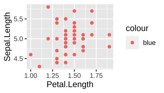
The right way to do this is
filter(iris, Species == "setosa") %>%
  ggplot(aes(x=Petal.Length, y = Sepal.Length)) +
    geom_point(color = "blue")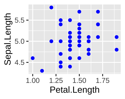
9.1.2.9.3 Fill vs color
There are two types of things to color in R – the fill argument fill space with a color and the color argument colors lines and points. To demonstrate let’s first make two histograms of Iris setosa sepal length with decorative color:
So we usually want to make histograms and density plots by specifying our desired color with fill. I usually add color = "white" to separate the bars in the histogram.*
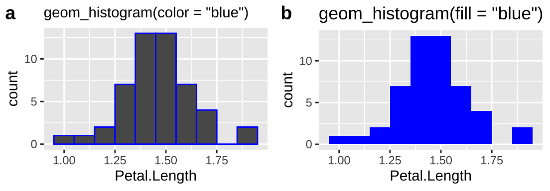
Now let’s try the same for color, now plotting petal length against sepal length, mapping species onto color or fill.
plotA <- ggplot(iris, aes(x=Petal.Length,  y = Sepal.Length, color = Species)) +
  geom_point()+   labs(title = 'aes(color = Species)')

plotB <- ggplot(iris, aes(x=Petal.Length, y = Sepal.Length, fill = Species)) +
  geom_point()+  labs(title = 'aes(fill = Species)')

# using plot_grid in the cowplot package to combine plots
plot_grid(plotA, plotB, labels = c("a","b"))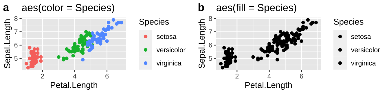
So we usually want to make scatterplots and lineplots by specifying our desired color with color.
9.1.2.9.4 Bar plots with count data
Imagine we wanted to plot hair color and eye color for men and women. Because this is count data, some form of bar chart would be good. If our data looks like this
We can make a bar plot with geom_bar
ggplot(hair_eye, aes(x = Sex, fill = Eye))+
  geom_bar(position = "fill", color = "white")+
  facet_wrap(~Hair, nrow = 1, labeller = "label_both")+
  scale_fill_manual(values = c("blue","brown","green","gold"))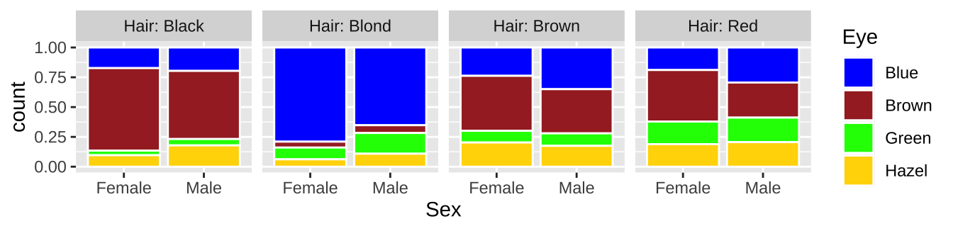
But if our data looked like this:
geom_bar would result in an error.
ggplot(HairEyeColor, aes(x = Sex, y = n, fill = Eye))+
  geom_bar(position = "fill", color = "white")+
  facet_wrap(~Hair, nrow = 1, labeller = "label_both")+
  scale_fill_manual(values = c("blue","brown","green","gold"))
## Error in `f()`:
## ! stat_count() can only have an x or y aesthetic.
We could overcome this error by using geom_col() instead of geom_bar(), or by typing geom_bar(position = "fill", color = "white", stat = 'identity').
9.1.2.10 When you give R a tibble
Throughout this course, we deal mostly with data in tibbles, a really nice way to store a bunch of variables of different classes – each as its own vector in a column. However occasionally we need to pull a vector from its tibble, to do so, type:
pull(.data = <name_of_tibble>, var = <name_of_column>)
## or
name_of_tibble %>%
  pull(var = name_of_column)
9.2 Making Reproducible examples to get help
In R it’s good to seek help, but great to help people help you. Watch this video on making reproducible examples, so that people can help you with your R (or you can help yourself)
9.3 Readable and usable R code
Remember - major benefit of R or any scripting language over e.g. doing a bunch of calculations in an excel are
- You have a record of exactly what you did,
- Which you can share with others,
- And/or you can update / change as your analyses progress.
For this reason it is important to have reliable a way to go from the R code you wrote one day to the output you got that day. There are two broad strategies you could take to accomplish this – your could save your works as a well organized script or you could write your code in RMarkdown (or comparably as an RNotebook). I discuss how to do each below.
9.3.1 Saving well-organized R scripts
Saving your R script is a great way to keep a shareable, replicable, reusable and editable record of what you have done. However, simply saving your R script does not guarantee that you will achieve these goals. Below I have some tips about what to include in your R script what to exclude, and examples of good and bad R scripts.
9.3.1.1 Things that should be in an R script
An R script should have all the commands and variable assignments etc that are necessary to reproduce your results. This includes loading the appropriate libraries, data sets etc etc etc.
Additionally, saved R scripts should be heavily commented (remember that comments start with # to tell R that were not writing code). Our goal here is not just that someone could run our code and get our result, but they could understand the intermediate steps ad why we did them.
9.3.1.2 Things that should not be in an R script
Because we will often share our R scripts with others, it is generally bad practice to point to your home directory (that is, use R projects rather than setwd()).
It is also considered unfriendly to begin your code by clearing R’s memory (do not start your code with rm(list = ls())). If you want to clear R’s memory (which is often a very good idea), type rm(list = ls()) in the console rather than in your saved script.
Additionally, you should only have commands in your saved scripts that are necessary to get through your analysis. So, for example, although we should use the glimpse() and view() functions extensively as we develop our analysis there is no reason to include these functions in the code you save.
9.3.1.3 Examples of good and bad R scripts
So our goal in writing an R script is not just to have it work immediately, but to (1) have it work if we exited R, reopened it, and ran our code without thinking, and (2) Have a sense of what the code was trying to do and how it was trying to do it.
Here is a bad R script. Note that this does not state our goal, it does not load the required library and it will not work if you simply run it. That is not to say this didn’t work when you first coded it – you could have had tidyverse loaded elsewhere, and you could have entered code into the console in an order which differed from how it is seen in you script. But it wont work as is.
mean_iris_sepal_length
mean_iris_sepal_length <- summarise(grouped_iris_data, mean(Sepal.Length))
grouped_iris_data      <- group_by(iris, Species)
Here is a good R script
# Yaniv Brandvain
# Feb 6 2022
# Calculating means with group_by

library(tidyverse) # load the tidyverse library

# Today our goal is to calculate the mean Sepal.Length
# for each species in the iris data set and save it to
# mean_iris_sepal_length
grouped_iris_data <- iris %>%  # Staring with iris dataset
  group_by(Species)            # When dealing with this tibble, do commands separately for each Species

mean_iris_sepal_length  <- grouped_iris_data %>%
  summarise(mean_sepal_length = mean(Sepal.Length)) # calculate the mean Sepal.Length

mean_iris_sepal_length # print our results to console
9.3.2 RMarkdown

RMarkdown is a file format that allows us to seamlessly combine text, R Code, results and plots. You use RMarkdown by writing in plain text and then interspersed with code chunks. See the video below (9.3) for a brief overview.
Figure 9.3: A brief (4 min and 37 sec) overview of RMarkdown from Stat 545.
You can use RMarkdown to make pdfs, html, or word documents that you can share with peers, employers etc… RMardown is especially useful for communicating results of complex data analysis, as your numbers, figures, and code will all match. This also means that anyone (especially future you, See Fig. 9.4) can recreate, learn from, and build off of your work.
Figure 9.4: Why make a reproducible workflow (A dramatic 1 min and 44 sec video).
Many students in this course like to turn in their homeworks as html documents generated by RMarkdown, because they can share their code, figures and ideas all in one place. Outside of class, the benefits are similar – people can see your code and results as they read your explanation. RMarkdown is pretty flexible – you can write lab reports, scientific papers, or even this book in RMarkdown.
To get started with RMarkdown, I suggest click File > New File > RMarkdown and start exploring. For a longer introduction, check out Chapter 27 of R for Data Science (Grolemund and Wickham 2018). Push onto Chapter 2 of RMarkdown: The definitive guide (Xie, Allaire, and Grolemund 2018) to dig even deeper.
A few RMarkdown tips:
You can control figure size by specifying
fig.heightandfig.widthand you can show the code or not with theecho = TRUEorecho = FALSEoptions in the beginning of your codechunk{r, fig.height = ..., fig.width = ..., echo = ...}).The
DTandkableExtrapackages can help make prettier tables.
If you have the time and energy, I strongly recommend that you turn in your first homework as an html generated by RMarkdown.
](https://d33wubrfki0l68.cloudfront.net/374f4c769f97c4ded7300d521eb59b24168a7261/c72ad/lesson-images/cheatsheets-1-cheatsheet.png)
Figure 9.5: download the RMarkdown cheat sheet