3.4 Transform a numeric variable

You can use any R arithmetic function to transform a continuous variable. For example, suppose you want to create a variable that is the square of another variable (e.g., to use a quadratic polynomial in a linear regression).

mydat$Yrs_From_Dx_2 <- mydat$Yrs_From_Dx^2

# Before vs. after
summary(mydat$Yrs_From_Dx)

##    Min. 1st Qu.  Median    Mean 3rd Qu.    Max.    NA's 
##     0.0     2.0     6.0     8.4    10.0    69.0      15

summary(mydat$Yrs_From_Dx_2)

##    Min. 1st Qu.  Median    Mean 3rd Qu.    Max.    NA's 
##       0       4      36     157     100    4761      15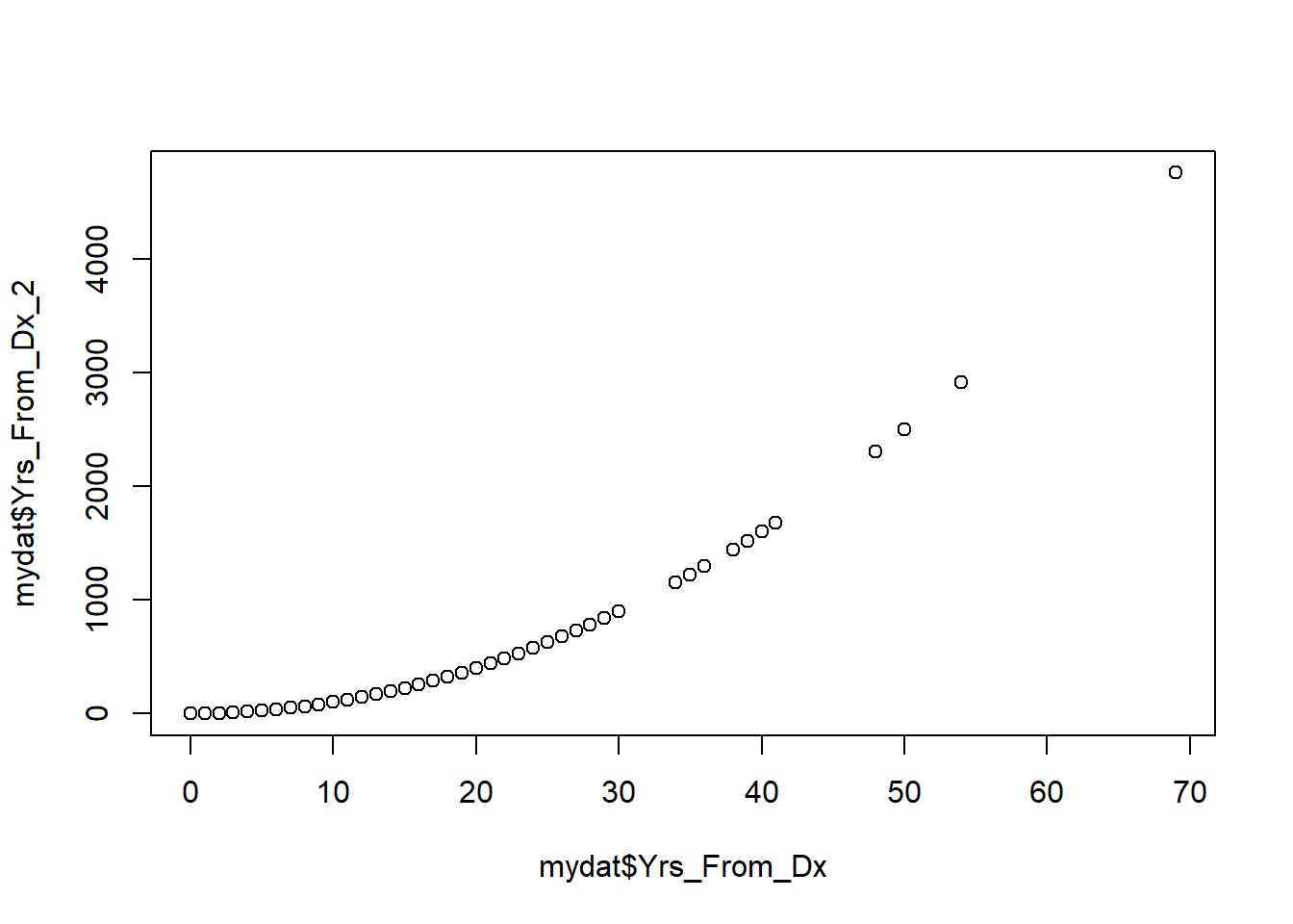

plot(mydat$Yrs_From_Dx, mydat$Yrs_From_Dx_2)

The tidyverse code to transform a variable uses the mutate() function.

mydat_tibble <- mydat_tibble %>% 
  mutate(Yrs_From_Dx_2 = Yrs_From_Dx^2)

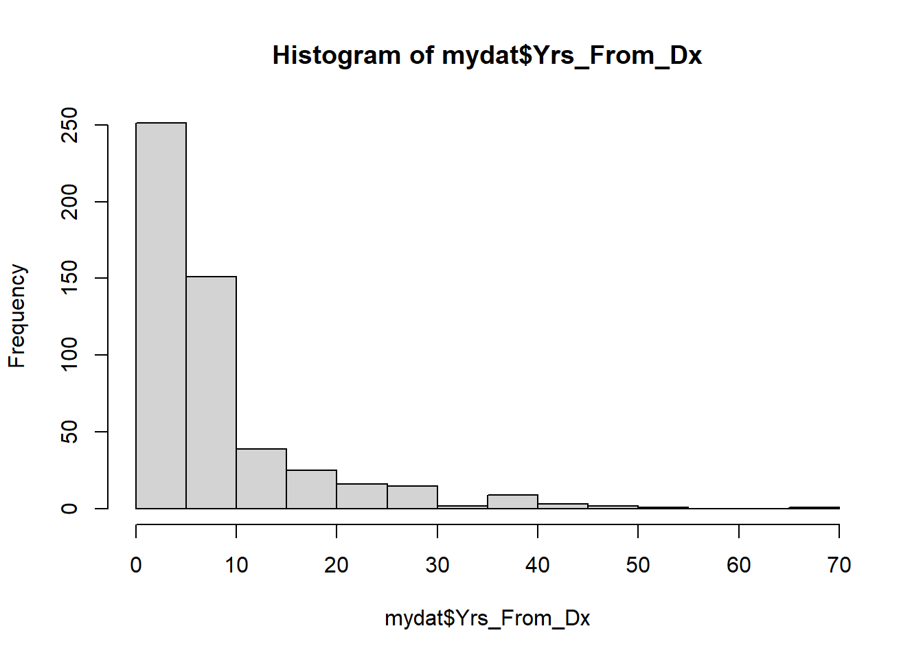
Another a common transformation is the log-transformation (usually the natural logarithm) for continuous variables that are skewed to the right. Many variables that represent time or size have a highly skewed distribution. When using a log-transformation, always check for zeros and negative numbers prior to transformation – log(0) is undefined and R will return a value of -Inf, log(-1) (or log of any negative number) is also undefined and will return a value of NaN along with a warning. You do not want a transformation that turns legitimate values into infinite or missing values.

If the original variable x is always positive then you can use log(x) directly. If x has some 0 values, then add a small number before transforming. Start with log(x + 1), but sometimes a larger or smaller number works better. Decide by looking at a histogram after the transformation. If the bar on the far left is far away from the other bars, consider adding a different number; for example, log(x + 10) or log(x + 0.1). If x has many zero values, or any negative values, a log-transformation might not be the best choice.

hist(mydat$Yrs_From_Dx)    # Very skewed

summary(mydat$Yrs_From_Dx) # There are zeros, so add 1

##    Min. 1st Qu.  Median    Mean 3rd Qu.    Max.    NA's 
##     0.0     2.0     6.0     8.4    10.0    69.0      15

mydat$log_Yrs_From_Dx <- log(mydat$Yrs_From_Dx + 1)

# NOTE: log() is the natural log
hist(mydat$log_Yrs_From_Dx) # More symmetric, bar at the left not far away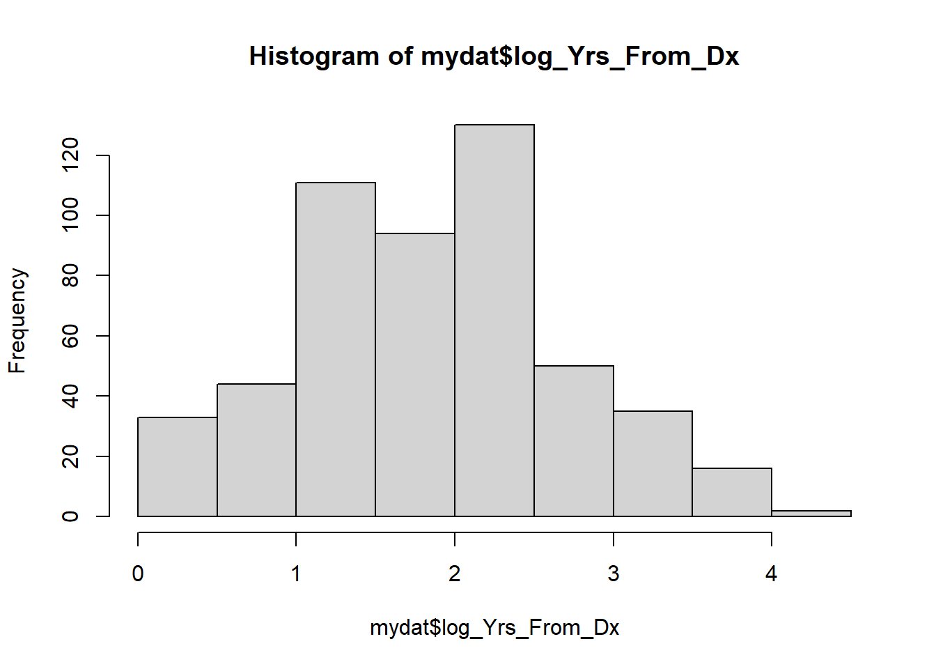

In this case log(x + 1) worked, but in other cases you may need a different number.

# If you had added too large a number, still too skewed
hist(log(mydat$Yrs_From_Dx + 10))

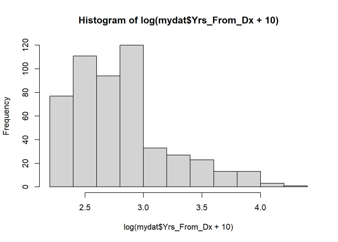
# If you had added too small a number,
# the bar to the left would be too far away from the rest of the data
hist(log(mydat$Yrs_From_Dx + 0.1))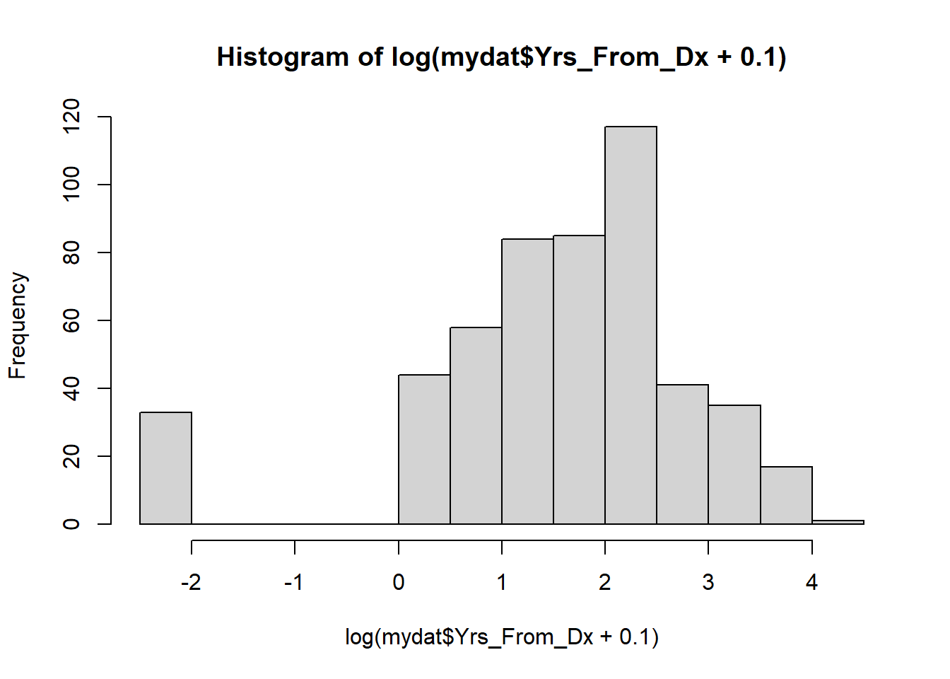

The tidyverse code for a log-transformation:

# Very skewed
mydat_tibble %>% 
  ggplot(aes(x = Yrs_From_Dx)) +
  geom_histogram(bins = 10, color="black", fill="white") +
  labs(y = "Frequency", x = "Years from Diagnosis")

summary(mydat$Yrs_From_Dx)

# There are zeros, so add 1
mydat_tibble <- mydat_tibble %>% 
  mutate(log_Yrs_From_Dx = log(Yrs_From_Dx + 1))

# NOTE: log() is the natural log
# More symmetric, bar at the left not far away
mydat_tibble %>% 
  ggplot(aes(x = log_Yrs_From_Dx)) +
  geom_histogram(bins = 10, color="black", fill="white") +
  labs(y = "Frequency", x = "log(Years from Diagnosis + 1)")