2.6 Inspecting the data
NOTE: This is just an overview of how to inspect the data for anomalies. More detail on descriptive statistics and data visualization will be given in Chapters 5 and 6, respectively, including a wider variety of methods and customization options.
DO: Open the file RheumArth_Tx_AgeComparisons_Data Dictionary.pdf. It contains variable definitions for the Rheumatoid Arthritis (RheumArth) dataset.
2.6.1 Base R
DO: Import RheumArth-Modified.csv using the base R function read.csv
What are the numbers of rows and columns in this dataset?
## [1] 530 14What are the variable names?
##  [1] "ID"            "Age"           "AgeGp"         "Sex"           "Yrs_From_Dx"
##  [6] "CDAI"          "CDAI_YN"       "DAS_28"        "DAS28_YN"      "Steroids_GT_5"
## [11] "DMARDs"        "Biologics"     "sDMARDS"       "OsteopScreen"
What is the type of each variable? This uses the lapply() function, which applies a function to each element of a list (recall that a data.frame is also a list). The unlist() function converts the output list to a vector (in this case, used just to make the output easier to view).
##            ID           Age         AgeGp           Sex   Yrs_From_Dx          CDAI
##     "integer"     "integer"     "integer"     "integer"     "integer"     "numeric"
##       CDAI_YN        DAS_28      DAS28_YN Steroids_GT_5        DMARDs     Biologics
##   "character"     "numeric"     "integer"     "integer"     "integer"     "integer"
##       sDMARDS  OsteopScreen
##     "integer"     "integer"
Some variables were read as integers, others as numeric. Look at the first 10 rows.
##    ID Age AgeGp Sex Yrs_From_Dx CDAI CDAI_YN DAS_28 DAS28_YN Steroids_GT_5 DMARDs
## 1   1  85     2   0          27   NA       1     NA        1             0      1
## 2   2  86     2   0          27 23.0       Y     NA        1             1      1
## 3   3  83     2   0          10 14.5       2     NA        1             1      1
## 4   4  83     2   0           9   NA       1     NA        1             1      1
## 5   5  85     2   0          NA   NA       1     NA        1             0      0
## 6   6  79     2   1          NA   NA       1     NA        1             0      0
## 7   7  90     2   0          51   NA       1     NA        1             0      1
## 8   8  90     2   0          11 40.0       2     NA        1             1      0
## 9   9  87     2   0          36  6.0       2     NA        1             0      0
## 10 10  82     2   0           4   NA       1     NA        1             0      1
##    Biologics sDMARDS OsteopScreen
## 1          0       0            0
## 2          0       0            1
## 3          1       0            1
## 4          0       0            1
## 5          0       0            0
## 6          0       0            0
## 7          1       0            0
## 8          0       0            1
## 9          1       0            1
## 10         0       0            1
2.6.1.1 Tabular inspection
It is useful to get a quick overview of each variable in the dataset. The first thing I want to see are all the possible values in a frequency table. For example, for AgeGp:
# useNA = "ifany" tells table() to display the number missing values if there are any
table(RheumArth$AgeGp, useNA = "ifany")
##
## 1 2 3
## 459 70 1There are lots of 1s and 2s, but also a 3. What does the codebook say about this variable?
- 1 = 40 to 70 years (“control”)
- 2 = 75 and older (“elderly”)
This implies 3 is an invalid value. Here is how to set this value to missing (see also Section 3.7).
# Set a value to missing
# Store a copy of the original variable
RheumArth$AgeGp_orig <- RheumArth$AgeGp
# Set values that are not 1 or 2 to missing
RheumArth$AgeGp[!(RheumArth$AgeGp %in% c(1, 2))] <- NA
# Table the new variable
table(RheumArth$AgeGp, useNA = "ifany")##
## 1 2 <NA>
## 459 70 1##
## 1 2 <NA>
## 1 459 0 0
## 2 0 70 0
## 3 0 0 1The old value of 3 is now NA.
NOTE: Instead of using the condition !(RheumArth$AgeGp %in% c(1, 2)), I could have used the condition RheumArth$AgeGp == 3. But I know from the codebook that the only valid values are 1 and 2, so the code I used can set all invalid value to missing, not just 3. Also, I wanted to illustrate the use of “not” ! with %in%. There is no “not in” operator, so I put the ! operator in front of the opposite condition in parentheses.
I am going to write a loop to display the tables for the rest of the variables. I have to use print() because when inside a loop the table() function does not display anything. I also print the name of each variable before its table. Within each table, the first row is the possible values and below that are the number of occurrences of each value.
# Use a loop to see the distribution of every variable in a dataset
for(i in 1:ncol(RheumArth)) {
print(names(RheumArth)[i])
print(table(RheumArth[, i], useNA = "ifany"))
cat("\n") # Adds a line before the next iteration
} ## [1] "ID"
##
## 1 2 3 4 5 6 7 8 9 10 11 12 13 14 15 16 17 18 19 20 21
## 1 1 1 1 1 1 1 1 1 1 1 1 1 1 1 1 1 1 1 1 1
## 22 23 24 25 26 27 28 29 30 31 32 33 34 35 36 37 38 39 40 41 42
## 1 1 1 1 1 1 1 1 1 1 1 1 1 1 1 1 1 1 1 1 1
## 43 44 45 46 47 48 49 50 51 52 53 54 55 56 57 58 59 60 61 62 63
## 1 1 1 1 1 1 1 1 1 1 1 1 1 1 1 1 1 1 1 1 1
## 64 65 66 67 68 69 70 71 101 102 103 104 105 106 107 108 109 110 111 112 113
## 1 1 1 1 1 1 1 1 1 1 1 1 1 1 1 1 1 1 1 1 1
## 114 115 116 117 118 119 120 121 122 123 124 125 126 127 128 129 130 131 132 133 134
## 1 1 1 1 1 1 1 1 1 1 1 1 1 1 1 1 1 1 1 1 1
## 135 136 137 138 139 140 141 142 143 144 145 146 147 148 149 150 151 152 153 154 155
## 1 1 1 1 1 1 1 1 1 1 1 1 1 1 1 1 1 1 1 1 1
## 156 157 158 159 160 161 162 163 164 165 166 167 168 169 170 171 172 173 174 175 176
## 1 1 1 1 1 1 1 1 1 1 1 1 1 1 1 1 1 1 1 1 1
## 177 178 179 180 181 182 183 184 185 186 187 188 189 190 191 192 193 194 195 196 197
## 1 1 1 1 1 1 1 1 1 1 1 1 1 1 1 1 1 1 1 1 1
## 198 199 200 201 202 203 204 205 206 207 208 209 210 211 212 213 214 215 216 217 218
## 1 1 1 1 1 1 1 1 1 1 1 1 1 1 1 1 1 1 1 1 1
## 219 220 221 222 223 224 225 226 227 228 229 230 231 232 233 234 235 236 237 238 239
## 1 1 1 1 1 1 1 1 1 1 1 1 1 1 1 1 1 1 1 1 1
## 240 241 242 243 244 245 246 247 248 249 250 251 252 253 254 255 256 257 258 259 260
## 1 1 1 1 1 1 1 1 1 1 1 1 1 1 1 1 1 1 1 1 1
## 261 262 263 264 265 266 267 268 269 270 271 272 273 274 275 276 277 278 279 280 281
## 1 1 1 1 1 1 1 1 1 1 1 1 1 1 1 1 1 1 1 1 1
## 282 283 284 285 286 287 288 289 290 291 292 293 294 295 296 297 298 299 300 301 302
## 1 1 1 1 1 1 1 1 1 1 1 1 1 1 1 1 1 1 1 1 1
## 303 304 305 306 307 308 309 310 311 312 313 314 315 316 317 318 319 320 321 322 323
## 1 1 1 1 1 1 1 1 1 1 1 1 1 1 1 1 1 1 1 1 1
## 324 325 326 327 328 329 330 331 332 333 334 335 336 337 338 339 340 341 342 343 344
## 1 1 1 1 1 1 1 1 1 1 1 1 1 1 1 1 1 1 1 1 1
## 345 346 347 348 349 350 351 352 353 354 355 356 357 358 359 360 361 362 363 364 365
## 1 1 1 1 1 1 1 1 1 1 1 1 1 1 1 1 1 1 1 1 1
## 366 367 368 369 370 371 372 373 374 375 376 377 378 379 380 381 382 383 384 385 386
## 1 1 1 1 1 1 1 1 1 1 1 1 1 1 1 1 1 1 1 1 1
## 387 388 389 390 391 392 393 394 395 396 397 398 399 400 401 402 403 404 405 406 407
## 1 1 1 1 1 1 1 1 1 1 1 1 1 1 1 1 1 1 1 1 1
## 408 409 410 411 412 413 414 415 416 417 418 419 420 421 422 423 424 425 426 427 428
## 1 1 1 1 1 1 1 1 1 1 1 1 1 1 1 1 1 1 1 1 1
## 429 430 431 432 433 434 435 436 437 438 439 440 441 442 443 444 445 446 447 448 449
## 1 1 1 1 1 1 1 1 1 1 1 1 1 1 1 1 1 1 1 1 1
## 450 451 452 453 454 455 456 457 458 459 460 461 462 463 464 465 466 467 468 469 470
## 1 1 1 1 1 1 1 1 1 1 1 1 1 1 1 1 1 1 1 1 1
## 471 472 473 474 475 476 477 478 479 480 481 482 483 484 485 486 487 488 489 490 491
## 1 1 1 1 1 1 1 1 1 1 1 1 1 1 1 1 1 1 1 1 1
## 492 493 494 495 496 497 498 499 500 501 502 503 504 505 506 507 508 509 510 511 512
## 1 1 1 1 1 1 1 1 1 1 1 1 1 1 1 1 1 1 1 1 1
## 513 514 515 516 517 518 519 520 521 522 523 524 525 526 527 528 529 530 531 532 533
## 1 1 1 1 1 1 1 1 1 1 1 1 1 1 1 1 1 1 1 1 1
## 534 535 536 537 538 539 540 541 542 543 544 545 546 547 548 549 550 551 552 553 554
## 1 1 1 1 1 1 1 1 1 1 1 1 1 1 1 1 1 1 1 1 1
## 555 556 557 558 559
## 1 1 1 1 1
##
## [1] "Age"
##
## 42 43 44 45 46 47 48 49 50 51 52 53 54 55 56 57 58 59 60 61 62
## 6 2 8 8 7 14 10 9 13 18 17 20 29 24 14 20 25 22 25 27 16
## 63 64 65 66 67 68 69 70 75 76 77 78 79 80 81 82 83 84 85 86 87
## 21 18 17 17 11 18 12 9 3 9 11 3 4 6 3 4 5 4 3 3 3
## 88 90 999
## 2 7 3
##
## [1] "AgeGp"
##
## 1 2 <NA>
## 459 70 1
##
## [1] "Sex"
##
## 0 1
## 428 102
##
## [1] "Yrs_From_Dx"
##
## -7 1 2 3 4 5 6 7 8 9 10 11 12 13 14 15 16
## 1 33 44 58 53 31 32 30 22 26 47 25 10 9 4 10 6
## 17 18 19 20 21 22 23 24 25 26 27 28 29 30 31 35 36
## 2 8 7 4 4 2 4 3 5 2 3 3 1 5 3 1 1
## 37 39 40 41 42 49 51 55 70 <NA>
## 1 1 6 1 3 1 1 1 1 15
##
## [1] "CDAI"
##
## 0 1 1.5 2 3 4 5 6 7 7.5 8 8.5 9 9.5 10 11 12
## 14 4 1 7 4 8 8 12 8 1 15 1 15 1 11 6 7
## 13 13.5 14 14.5 15 16 17 18 19 20 21 22 23 24 25 28 31
## 5 1 8 1 4 6 8 4 6 5 3 3 3 2 1 3 1
## 32 34 35 36 37 39 39.5 40 40.5 41 51 71 <NA>
## 2 1 2 1 2 4 1 2 1 1 1 1 324
##
## [1] "CDAI_YN"
##
## 1 2 Y
## 324 205 1
##
## [1] "DAS_28"
##
## 0 0.46 0.56 0.77 0.84 0.97 1.05 1.27 1.3 1.4 1.51 1.53 1.54 1.7 1.82 1.84 1.87
## 1 1 1 1 1 1 1 1 1 1 1 1 2 1 2 1 1
## 1.94 2.1 2.2 2.3 2.34 2.37 2.39 2.44 2.46 2.49 2.5 2.52 2.68 2.82 2.84 2.87 2.97
## 1 2 1 1 1 2 2 1 1 1 2 2 1 1 1 1 1
## 3.02 3.03 3.04 3.09 3.1 3.16 3.28 3.32 3.44 3.73 3.8 3.94 4 4.01 4.04 4.21 4.28
## 2 1 1 1 1 1 1 1 1 1 1 1 1 1 1 1 1
## 4.39 4.48 4.49 4.68 4.8 5.65 23 <NA>
## 1 1 1 1 1 1 1 464
##
## [1] "DAS28_YN"
##
## 1 2
## 464 66
##
## [1] "Steroids_GT_5"
##
## 0 1 <NA>
## 405 124 1
##
## [1] "DMARDs"
##
## 0 1 <NA>
## 149 380 1
##
## [1] "Biologics"
##
## 0 1 <NA>
## 332 197 1
##
## [1] "sDMARDS"
##
## 0 1 <NA>
## 502 27 1
##
## [1] "OsteopScreen"
##
## 0 1 <NA>
## 216 306 8
##
## [1] "AgeGp_orig"
##
##   1   2   3
## 459 70 1Do you see any potential data anomalies?
DO: Before reading further, look at the tables above and note any values that appear strange to you.
The potential anomalies I see are the following:
Agehas some values that are 999Yrs_From_Dxhas a value of -7CDAIhas 14 zerosCDAI_YNhas mostly 1s and 2s but also a YDAS_28has a zero- Both
CDAIandDAS_28have many missing values
Looking at the codebook leads to the following conclusions:
Age= 999 is probably a missing value code. Typically, such codes would be specified in the codebook. In this case, I modified the data myself for this example so this is not in the codebook. Either way, these values should be set to NA (missing).Yrs_From_Dxshould not have any negative values. It is possible this was a data entry error and should be 7 instead of -7. If you had access to the data collection team, you could ask. Otherwise, probably best to set it to missing.- Zero values are valid for
CDAI. No change needed. - The
YforCDAI_YNcan be assumed to mean “Yes” and be recoded as a 2. - The codebook is not clear regarding whether
DAS_28can be zero, saying only that < 2.6 indicates remission. While it seems odd that there is only one zero,DAS_28is a score so a zero is plausible. You could do some further searching for “disease activity score” online to see if zeros really are allowed. - For
CDAIandDAS_28, the codebook states that “Blanks are informative missing, as they indicate tests not given, rather than unknown.”
You can use summary() to summarize a numeric variable. Look at the summaries of CDAI and DAS_28 by values of their corresponding _YN variables, which indicate whether a test was given. The following is for DAS_28; you can imitate this code for CDAI, as well.
##    Min. 1st Qu.  Median    Mean 3rd Qu.    Max.    NA's
##    0.00    1.82    2.50    2.92    3.31   23.00     464
# tapply applies a function to one variable at every level of another
tapply(RheumArth$DAS_28, RheumArth$DAS28_YN, summary) ## $`1`
## Min. 1st Qu. Median Mean 3rd Qu. Max. NA's
## NA NA NA NaN NA NA 464
##
## $`2`
## Min. 1st Qu. Median Mean 3rd Qu. Max.
## 0.00 1.82 2.50 2.92 3.31 23.00- At
DAS28_YN= 1 (No),DAS_28is always missing. These are the individuals not given this test. - At
DAS28_YN= 2 (Yes),DAS_28has no missing values, and ranges from 0 to 23 with a mean of 2.923.
The summary() function can also be used on the entire dataset to summarize all variables at once.
##        ID           Age          AgeGp           Sex         Yrs_From_Dx
##  Min.   :  1   Min.   : 42   Min.   :1.00   Min.   :0.000   Min.   :-7.00
##  1st Qu.:162   1st Qu.: 54   1st Qu.:1.00   1st Qu.:0.000   1st Qu.: 3.00
##  Median :294   Median : 59   Median :1.00   Median :0.000   Median : 7.00
##  Mean   :291   Mean   : 66   Mean   :1.13   Mean   :0.192   Mean   : 9.37
##  3rd Qu.:427   3rd Qu.: 66   3rd Qu.:1.00   3rd Qu.:0.000   3rd Qu.:11.00
##  Max.   :559   Max.   :999   Max.   :2.00   Max.   :1.000   Max.   :70.00
##                              NA's   :1                      NA's   :15
##       CDAI        CDAI_YN              DAS_28         DAS28_YN    Steroids_GT_5
##  Min.   : 0.0   Length:530         Min.   : 0.00   Min.   :1.00   Min.   :0.000
##  1st Qu.: 6.0   Class :character   1st Qu.: 1.82   1st Qu.:1.00   1st Qu.:0.000
##  Median :10.0   Mode  :character   Median : 2.50   Median :1.00   Median :0.000
##  Mean   :13.1                      Mean   : 2.92   Mean   :1.12   Mean   :0.234
##  3rd Qu.:17.0                      3rd Qu.: 3.31   3rd Qu.:1.00   3rd Qu.:0.000
##  Max.   :71.0                      Max.   :23.00   Max.   :2.00   Max.   :1.000
##  NA's   :324                       NA's   :464                    NA's   :1
##      DMARDs        Biologics        sDMARDS       OsteopScreen     AgeGp_orig
##  Min.   :0.000   Min.   :0.000   Min.   :0.000   Min.   :0.000   Min.   :1.00
##  1st Qu.:0.000   1st Qu.:0.000   1st Qu.:0.000   1st Qu.:0.000   1st Qu.:1.00
##  Median :1.000   Median :0.000   Median :0.000   Median :1.000   Median :1.00
##  Mean   :0.718   Mean   :0.372   Mean   :0.051   Mean   :0.586   Mean   :1.14
##  3rd Qu.:1.000   3rd Qu.:1.000   3rd Qu.:0.000   3rd Qu.:1.000   3rd Qu.:1.00
##  Max.   :1.000   Max.   :1.000   Max.   :1.000   Max.   :1.000   Max.   :3.00
##  NA's   :1       NA's   :1       NA's   :1       NA's   :8
Even more informative is the describe() function in the Hmisc library (Harrell Jr, Charles Dupont, and others. 2021) for producing summaries of all variables in a dataset all at once. In the code below, we use the :: syntax to call a function from a library without loading the entire library.
## RheumArth
##
##  15  Variables      530  Observations
## -------------------------------------------------------------------------------------
## ID
##        n  missing distinct     Info     Mean  pMedian      Gmd      .05      .10
##      530        0      530        1    290.6      291    183.7    27.45    53.90
##      .25      .50      .75      .90      .95
##   162.25   294.50   426.75   506.10   532.55
##
## lowest :   1   2   3   4   5, highest: 555 556 557 558 559
## -------------------------------------------------------------------------------------
## Age
##        n  missing distinct     Info     Mean  pMedian      Gmd      .05      .10
##      530        0       45    0.999    65.97       60    22.01       46       48
##      .25      .50      .75      .90      .95
##       54       59       66       77       83
##
## lowest :  42  43  44  45  46, highest:  86  87  88  90 999
## -------------------------------------------------------------------------------------
## AgeGp
##        n  missing distinct     Info     Mean
##      529        1        2    0.344    1.132
##
## Value          1     2
## Frequency    459    70
## Proportion 0.868 0.132
## -------------------------------------------------------------------------------------
## Sex
##        n  missing distinct     Info      Sum     Mean
##      530        0        2    0.466      102   0.1925
##
## -------------------------------------------------------------------------------------
## Yrs_From_Dx
##        n  missing distinct     Info     Mean  pMedian      Gmd      .05      .10
##      515       15       43    0.995    9.373      7.5    8.802      1.0      2.0
##      .25      .50      .75      .90      .95
##      3.0      7.0     11.0     21.0     29.3
##
## lowest : -7  1  2  3  4, highest: 42 49 51 55 70
## -------------------------------------------------------------------------------------
## CDAI
##        n  missing distinct     Info     Mean  pMedian      Gmd      .05      .10
##      206      324       46    0.998     13.1     11.5     11.4      0.0      2.0
##      .25      .50      .75      .90      .95
##      6.0     10.0     17.0     28.0     38.5
##
## lowest : 0    1    1.5  2    3   , highest: 40   40.5 41   51   71
## -------------------------------------------------------------------------------------
## CDAI_YN
##        n  missing distinct
##      530        0        3
##
## Value          1     2     Y
## Frequency    324   205     1
## Proportion 0.611 0.387 0.002
## -------------------------------------------------------------------------------------
## DAS_28
##        n  missing distinct     Info     Mean  pMedian      Gmd      .05      .10
##       66      464       58        1    2.923     2.63    1.923   0.7875   1.1600
##      .25      .50      .75      .90      .95
##   1.8250   2.5000   3.3100   4.3350   4.6325
##
## lowest : 0    0.46 0.56 0.77 0.84, highest: 4.49 4.68 4.8  5.65 23
## -------------------------------------------------------------------------------------
## DAS28_YN
##        n  missing distinct     Info     Mean
##      530        0        2    0.327    1.125
##
## Value          1     2
## Frequency    464    66
## Proportion 0.875 0.125
## -------------------------------------------------------------------------------------
## Steroids_GT_5
##        n  missing distinct     Info      Sum     Mean
##      529        1        2    0.538      124   0.2344
##
## -------------------------------------------------------------------------------------
## DMARDs
##        n  missing distinct     Info      Sum     Mean
##      529        1        2    0.607      380   0.7183
##
## -------------------------------------------------------------------------------------
## Biologics
##        n  missing distinct     Info      Sum     Mean
##      529        1        2    0.701      197   0.3724
##
## -------------------------------------------------------------------------------------
## sDMARDS
##        n  missing distinct     Info      Sum     Mean
##      529        1        2    0.145       27  0.05104
##
## -------------------------------------------------------------------------------------
## OsteopScreen
##        n  missing distinct     Info      Sum     Mean
##      522        8        2    0.728      306   0.5862
##
## -------------------------------------------------------------------------------------
## AgeGp_orig
##        n  missing distinct     Info     Mean  pMedian      Gmd
##      530        0        3    0.348    1.136        1   0.2362
##
## Value          1     2     3
## Frequency    459    70     1
## Proportion 0.866 0.132 0.002
##
## For the frequency table, variable is rounded to the nearest 0
## -------------------------------------------------------------------------------------
2.6.1.2 Graphical inspection
You can also inspect the data graphically, as will be discussed in more detail in Chapter 6. For a variable with only a few levels, a bar chart is appropriate.
# Bar chart for a categorical variable
# barplot expects the frequencies, not the raw data, so use table inside barplot
barplot(table(RheumArth$AgeGp))
title("Age Group")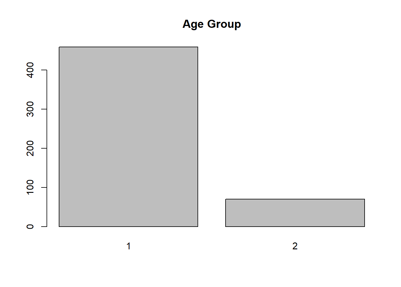
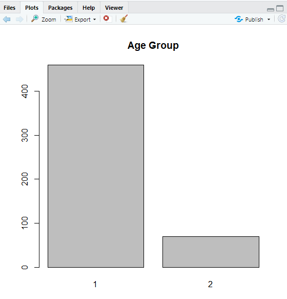
The output is shown in the lower right panel, in the Plots tab and you can use the arrow button to page through them.
The x-axis does not look right. AgeGp is not a continuous variable. It just has two levels, 1 = 40 to 70 years (“control”) and 2 = 75 and older (“elderly”). We can fix this by converting it to a factor before plotting. In Chapter 3, we will discuss how to clean up the data, including converting categorical variables to factors. If AgeGp were already a factor in the dataset, you would not need to convert it before plotting.
# If the variable is not already a factor, you can
# convert to a factor variable before plotting
# so the axis has appropriate labels
RheumArth$AgeGp = factor(RheumArth$AgeGp,
                        levels = 1:2,
                        labels = c("40-70y",
                                   "75y+"))
barplot(table(RheumArth$AgeGp))
title("Age Group")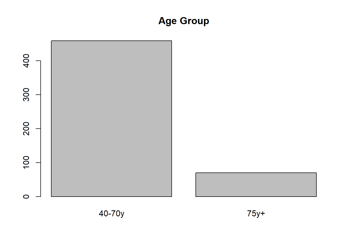
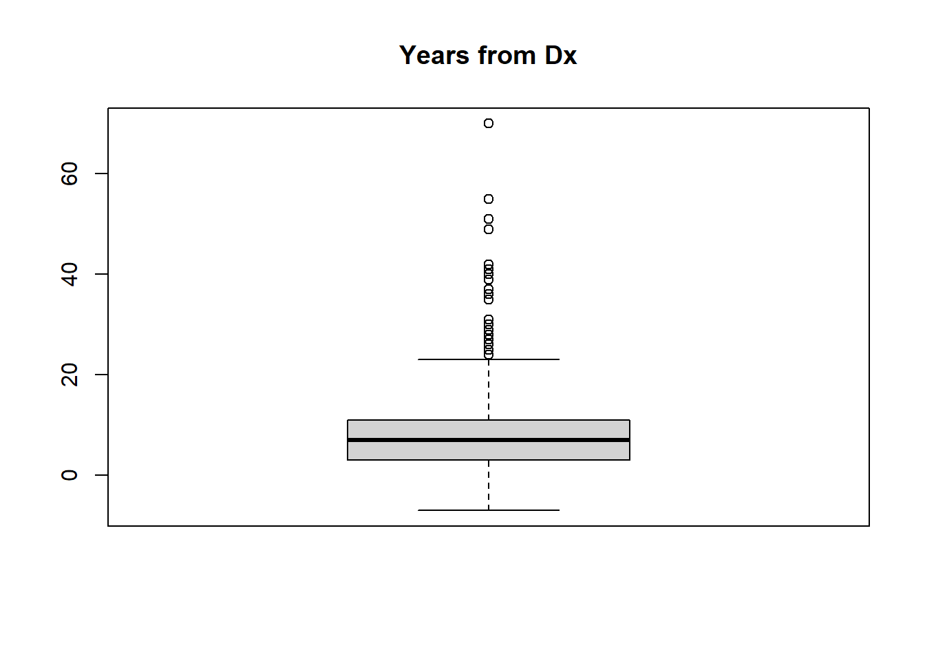
For a continuous variable, histograms and boxplots are appropriate.
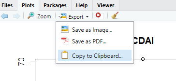
NOTE: You can copy a plot (to paste into a document) or save the plot as a file using the Export option in the Plots tab.
NOTE: One advantage of tabular summaries is that you can see the extent of missing data. A disadvantage is that other than numbers on the extremes it is not easy to see the overall distribution of the data. Use both tabular and graphical summaries –- that gives you the best chance of finding all data anomalies and understanding how each variable is distributed.
2.6.2 Tidyverse
The following contains tidyverse code for summarizing the data. Note the use of the “pipe” operator %>% which strings together functions operating on the same dataset.
DO: Import RheumArth-Modified.csv using the tidyverse function read_csv().
What are the numbers of rows and columns in this dataset? You could use dim() as before or, unlike with a data.frame, just enter the name of the tibble. This shows the first few rows (like head()) but also the dimensions (number of observations \(\times\) number of variables) and the type of each variable.
## # A tibble: 530 × 14
##       ID   Age AgeGp   Sex Yrs_From_Dx  CDAI CDAI_YN DAS_28 DAS28_YN Steroids_GT_5
##    <dbl> <dbl> <dbl> <dbl>       <dbl> <dbl> <chr>    <dbl>    <dbl>         <dbl>
##  1     1    85     2     0          27  NA   1           NA        1             0
##  2     2    86     2     0          27  23   Y           NA        1             1
##  3     3    83     2     0          10  14.5 2           NA        1             1
##  4     4    83     2     0           9  NA   1           NA        1             1
##  5     5    85     2     0          NA  NA   1           NA        1             0
##  6     6    79     2     1          NA  NA   1           NA        1             0
##  7     7    90     2     0          51  NA   1           NA        1             0
##  8     8    90     2     0          11  40   2           NA        1             1
##  9     9    87     2     0          36   6   2           NA        1             0
## 10    10    82     2     0           4  NA   1           NA        1             0
## # ℹ 520 more rows
## # ℹ 4 more variables: DMARDs <dbl>, Biologics <dbl>, sDMARDS <dbl>,
## #   OsteopScreen <dbl>
When there are many variables (many columns), they might not all be shown. To see all the variable names, use names(), and to see all the variable types, use spec() and str(). The spec() function shows you the variable specifications. The str() function gives the same information, plus a listing of the first few values for each variable.
##  [1] "ID"            "Age"           "AgeGp"         "Sex"           "Yrs_From_Dx"
##  [6] "CDAI"          "CDAI_YN"       "DAS_28"        "DAS28_YN"      "Steroids_GT_5"
## [11] "DMARDs" "Biologics" "sDMARDS" "OsteopScreen"## cols(
## ID = col_double(),
## Age = col_double(),
## AgeGp = col_double(),
## Sex = col_double(),
## Yrs_From_Dx = col_double(),
## CDAI = col_double(),
## CDAI_YN = col_character(),
## DAS_28 = col_double(),
## DAS28_YN = col_double(),
## Steroids_GT_5 = col_double(),
## DMARDs = col_double(),
## Biologics = col_double(),
## sDMARDS = col_double(),
## OsteopScreen = col_double()
## )## spc_tbl_ [530 × 14] (S3: spec_tbl_df/tbl_df/tbl/data.frame)
## $ ID : num [1:530] 1 2 3 4 5 6 7 8 9 10 ...
## $ Age : num [1:530] 85 86 83 83 85 79 90 90 87 82 ...
## $ AgeGp : num [1:530] 2 2 2 2 2 2 2 2 2 2 ...
## $ Sex : num [1:530] 0 0 0 0 0 1 0 0 0 0 ...
## $ Yrs_From_Dx : num [1:530] 27 27 10 9 NA NA 51 11 36 4 ...
## $ CDAI : num [1:530] NA 23 14.5 NA NA NA NA 40 6 NA ...
## $ CDAI_YN : chr [1:530] "1" "Y" "2" "1" ...
## $ DAS_28 : num [1:530] NA NA NA NA NA NA NA NA NA NA ...
## $ DAS28_YN : num [1:530] 1 1 1 1 1 1 1 1 1 1 ...
## $ Steroids_GT_5: num [1:530] 0 1 1 1 0 0 0 1 0 0 ...
## $ DMARDs : num [1:530] 1 1 1 1 0 0 1 0 0 1 ...
## $ Biologics : num [1:530] 0 0 1 0 0 0 1 0 1 0 ...
## $ sDMARDS : num [1:530] 0 0 0 0 0 0 0 0 0 0 ...
## $ OsteopScreen : num [1:530] 0 1 1 1 0 0 0 1 1 1 ...
## - attr(*, "spec")=
## .. cols(
## .. ID = col_double(),
## .. Age = col_double(),
## .. AgeGp = col_double(),
## .. Sex = col_double(),
## .. Yrs_From_Dx = col_double(),
## .. CDAI = col_double(),
## .. CDAI_YN = col_character(),
## .. DAS_28 = col_double(),
## .. DAS28_YN = col_double(),
## .. Steroids_GT_5 = col_double(),
## .. DMARDs = col_double(),
## .. Biologics = col_double(),
## .. sDMARDS = col_double(),
## .. OsteopScreen = col_double()
## .. )
## - attr(*, "problems")=<externalptr>2.6.2.1 Tabular inspection
Let’s get a quick overview of each variable in the dataset. To see all the possible values of a variable, use count(). This is similar to table(), except that the listing is vertical instead of horizontal and the number of missing values are included by default.
## # A tibble: 3 × 2
##   Biologics     n
##       <dbl> <int>
## 1         0   332
## 2         1   197
## 3        NA     1
NOTE: The pipe operator %>% allows you to string together commands. When using %>% you do not have to name the dataset in every command. The dataset appears only at the beginning of the pipe. In this example, there was only one command, but later examples will demonstrate the use of multiple commands strung together by multiple pipe operators.
If you wanted to save this table as an object, you would add a new object name with <- at the beginning like this:
## # A tibble: 3 × 2
##   AgeGp     n
##   <dbl> <int>
## 1     1   459
## 2     2    70
## 3     3     1
As before, we need to set the value AgeGp = 3 to missing. The mutate() function is used to manipulate variables. If you have more than one command, you can either include multiple commands separated by commas within one mutate() function call or string together multiple mutate() function calls using %>%.
# Set a value to missing
# Assign the object to itself or a new object
# (otherwise the changes you make will not be saved anywhere)
RheumArth_tibble <- RheumArth_tibble %>%
  # Store the original version of the variable
  # Replace specific value with NA
  mutate(AgeGp_orig = AgeGp,
         AgeGp = na_if(AgeGp, 3))

# Alternative with separate mutate calls
# RheumArth_tibble <- RheumArth_tibble %>%
#   # Store the original version of the variable
#   mutate(AgeGp_orig = AgeGp) %>%
#   # Replace specific value with NA
#   mutate(AgeGp = na_if(AgeGp, 3))

# Table the new variable
RheumArth_tibble %>%
  count(AgeGp)
## # A tibble: 3 × 2
## AgeGp n
## <dbl> <int>
## 1 1 459
## 2 2 70
## 3 NA 1## # A tibble: 3 × 3
## AgeGp_orig AgeGp n
## <dbl> <dbl> <int>
## 1 1 1 459
## 2 2 2 70
## 3 3 NA 1The count() function makes a table with 1 row for each unique combination of the variables. If you prefer a two-way table, use the base R function table().
# To get a two-way table, use table()
# Compare old to new
table(RheumArth_tibble$AgeGp_orig, RheumArth_tibble$AgeGp, useNA = "ifany")##
## 1 2 <NA>
## 1 459 0 0
## 2 0 70 0
## 3 0 0 1The na_if() function above replaced a specific value (3) with NA. The case_when() function is more general and can be used to replace values with NA if they meet a certain condition. It has a complicated syntax which we will cover more in depth in Section 3.1. Here we set any value that is not 1 or 2 to missing, otherwise (TRUE) leave the variable as is. In the first line, we must use as.double(NA) since AgeGp is numeric and stored as double, whereas NA is, by default, logical. If AgeGp were stored as integer, you would need to use as.integer(NA) instead.
# Re-load the data so AgeGp = 3 is present
RheumArth_tibble <- read_csv("Data/RheumArth-Modified.csv", na = c("NA", "."))
RheumArth_tibble <- RheumArth_tibble %>%
mutate(AgeGp_orig = AgeGp,
AgeGp = case_when(!(AgeGp %in% c(1, 2)) ~ as.double(NA),
TRUE ~ AgeGp))
# Compare old to new
RheumArth_tibble %>%
  count(AgeGp_orig, AgeGp)
## # A tibble: 3 × 3
## AgeGp_orig AgeGp n
## <dbl> <dbl> <int>
## 1 1 1 459
## 2 2 2 70
## 3 3 NA 1NOTE: For some purposes, the tidyverse method can be more complicated than the base R method, but there are other situations where the reverse is true. The goal here is to give you some background in both base R and tidyverse and then as you use R you can use whichever you prefer, and also be able to understand code written by others in either.
2.6.2.2 Graphical inspection
While base R uses a variety of functions like plot(), barplot(), hist(), etc., in tidyverse data visualization is generally done using ggplot(). We will go into more detail on the syntax in Chapter 6. For now, just note the following:
aes()stands for “aesthetic” and is where you tellggplot()what variables go on each axis and if there is a grouping variable.
For a variable with only a few levels, a bar chart is appropriate. As we did previously, we will convert AgeGp to a factor before plotting.
# Bar chart for a categorical variable
RheumArth_tibble %>%
  # Conversion to a factor only needed if the
  # variable is not already a factor
  mutate(AgeGp = factor(AgeGp,
                        levels = 1:2,
                        labels = c("40-70y",
                                   "75y+"))) %>%
  ggplot(aes(x = AgeGp)) +
  geom_bar() +
  labs(title = "Age Group", y = "Frequency")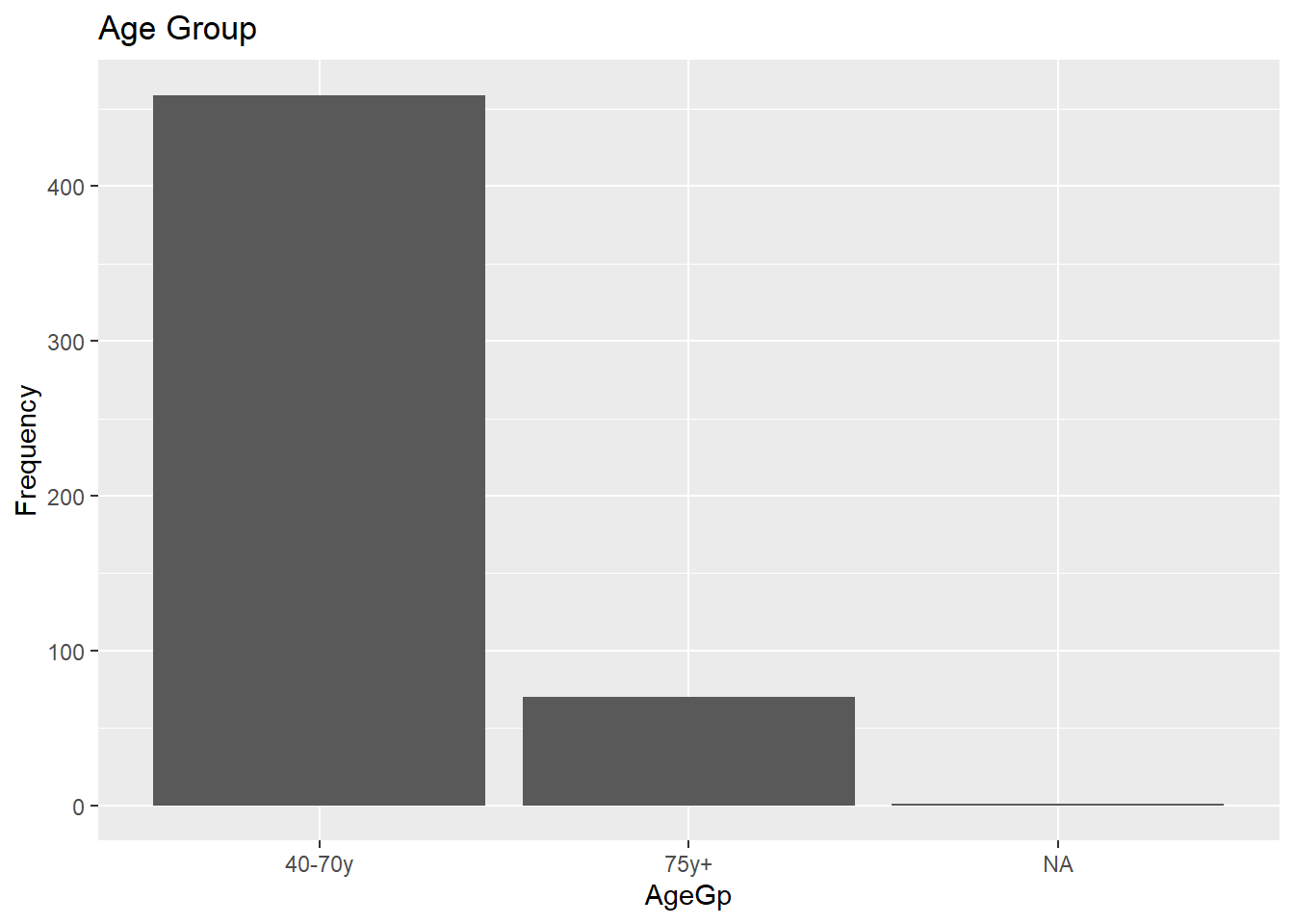
NOTE: When using ggplot(), you start with a dataset name, then use the pipe operator %>%, then ggplot(). To string together plotting statements after ggplot(), use plus signs +, not pipe operators.
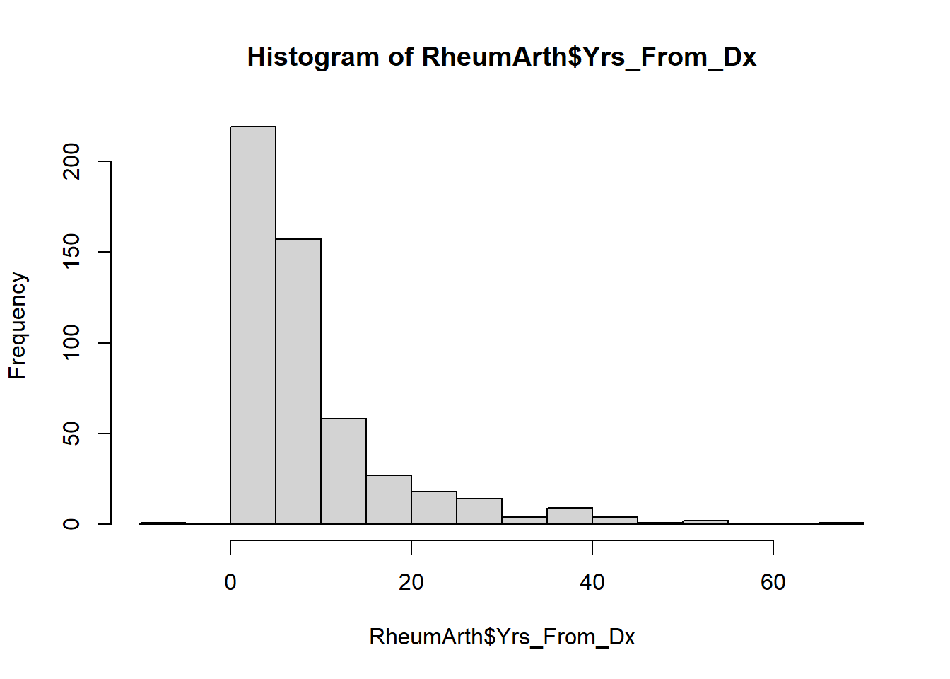
For a continuous variable, a histogram is appropriate.
# Histogram for a continuous variable
RheumArth_tibble %>%
  ggplot(aes(x = Yrs_From_Dx)) +
  geom_histogram() +
  labs(y = "Frequency", x = "Years from Diagnosis")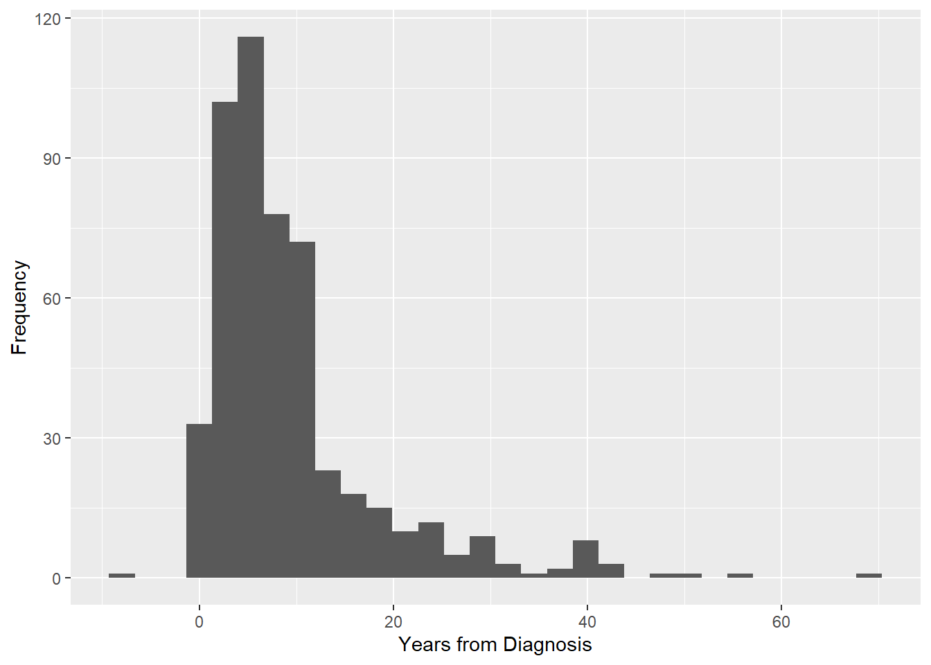
You may get some warnings when plotting a histogram.
- A note to “Pick better value with binwidth” has to do with how wide the bins are for the histogram. Wider bins result in a smoother histogram. You can ignore it, or change the value as shown below.
- A warning about rows being removed due to non-finite values is telling you that some values were not plotted because they were infinite or missing.
We can redo the histogram with a smaller number of bins. We also change the appearance of the histogram just to illustrate a few other options.
# Histogram for a continuous variable
# Set bins, bar color, bar fill
RheumArth_tibble %>%
  ggplot(aes(x = Yrs_From_Dx)) +
  geom_histogram(bins = 10, color="black", fill="white") +
  labs(y = "Frequency", x = "Years from Diagnosis")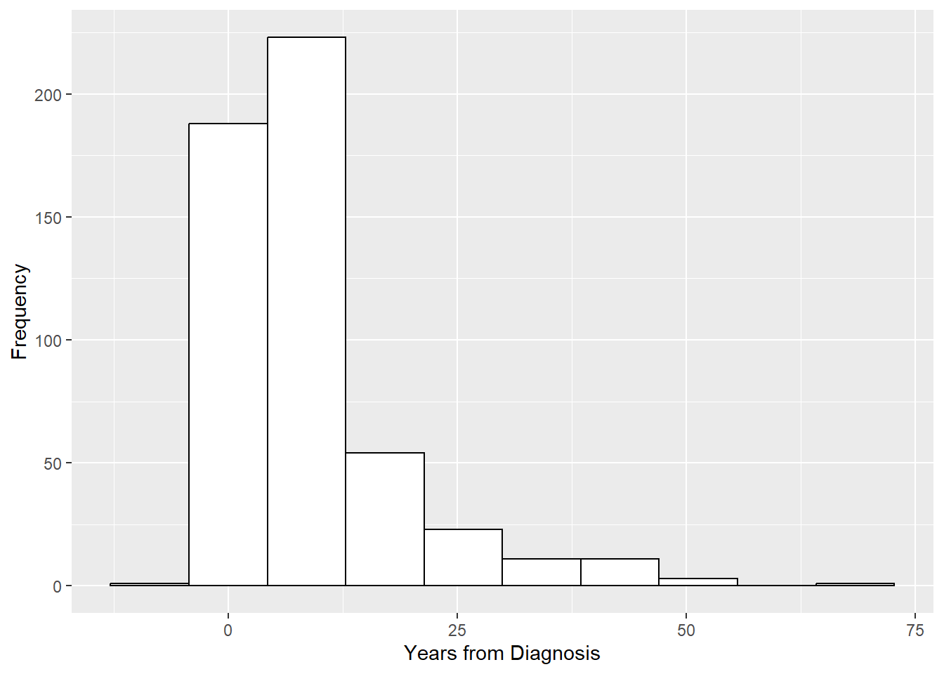
Boxplots are also appropriate for continuous variables. You can create vertical or horizontal boxplots
# Boxplot for a continuous variable
# Use y in aes and labs if you want a vertical boxplot
RheumArth_tibble %>%
  ggplot(aes(y = Yrs_From_Dx)) +
  geom_boxplot() +
  # Without these theme statements,
  # there will be a meaningless x-axis
  theme(axis.text.x  = element_blank(),
        axis.ticks.x = element_blank()) +
  labs(y = "Years from Diagnosis")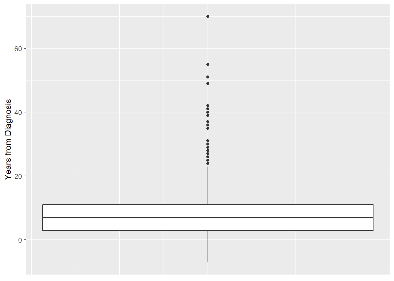
# Change the roles of x and y throughout
# if you want a horizontal boxplot
RheumArth_tibble %>%
  ggplot(aes(x = Yrs_From_Dx)) +
  geom_boxplot() +
  # Without these theme statements,
  # there will be a meaningless x-axis
  theme(axis.text.y  = element_blank(),
        axis.ticks.y = element_blank()) +
  labs(x = "Years from Diagnosis")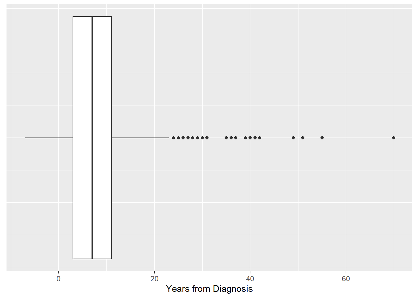
NOTE: ggplot() has a more complicated syntax than the base R plot functions, but unlike base R attempts to bring together many different visualizations into one consistent syntax. Both base R and ggplot() are powerful for plotting and it is worth learning both (see Chapter 6).