7.4 Prediction Analyses
In the previous section we described associational analyses, where the goal is to see if a key predictor \(x\) and an outcome \(y\) are associated. But sometimes the goal is to use all of the information available to you to predict \(y\). Furthermore, it doesn’t matter if the variables would be considered unrelated in a causal way to the outcome you want to predict because the objective is prediction, not developing an understanding about the relationships between features.
With prediction models, we have outcome variables–features about which we would like to make predictions–but we typically do not make a distinction between “key predictors” and other predictors. In most cases, any predictor that might be of use in predicting the outcome would be considered in an analysis and might, a priori, be given equal weight in terms of its importance in predicting the outcome. Prediction analyses will often leave it to the prediction algorithm to determine the importance of each predictor and to determine the functional form of the model.
For many prediction analyses it is not possible to literally write down the model that is being used to predict because it cannot be represented using standard mathematical notation. Many modern prediction routines are structured as algorithms or procedures that take inputs and transform them into outputs. The path that the inputs take to be transformed into outputs may be highly nonlinear and predictors may interact with other predictors on the way. Typically, there are no parameters of interest that we try to estimate–in fact many algorithmic procedures do not have any estimable parameters at all.
The key thing to remember with prediction analyses is that we usually do not care about the specific details of the model. In most cases, as long as the method “works”, is reproducible, and produces good predictions with minimal error, then we have achieved our goals.
With prediction analyses, the precise type of analysis you do depends on the nature of the outcome (as it does with all analyses). Prediction problems typically come in the form of a classification problem where the outcome is binary. In some cases the outcome can take more than two levels, but the binary case is by far the most common. In this section, we will focus on the binary classification problem.
7.4.0.1 Expectations
What’s the ideal scenario in a prediction problem? Generally, what we want is a predictor, or a set of predictors, to produce good separation in the outcome. Here’s an example of a single predictor producing reasonable separation in a binary outcome.
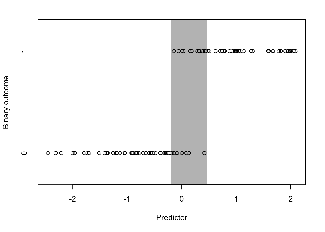
Figure 5.5: Ideal Classification Scenario
The outcome takes values of 0 and 1, while the predictor is continuous and takes values between roughly -2 and 2. The gray zone indicated in the plot highlights the area where values of the predictor can take on values of 0 or 1. To the right of the gray area you’ll notice that the value of the outcome is always 1 and to the left of the gray area the value of the outcome is always 0. In prediction problems, it’s this gray area where we have the most uncertainty about the outcome, given the value of the predictor.
The goal of most prediction problems to identify a set of predictors that minimizes the size of that gray area in the plot above. Counterintuitively, it is common to identify predictors (particularly categorical ones) that perfectly separate the outcome, so that the gray area is reduced to zero. However, such situations typically indicate a degenerate problem that is not of much interest or even a mistake in the data. For example, a continuous variable that has been dichotomized will be perfectly separated by its continuous counterpart. It is a common mistake to include the continuous version as a predictor in the model and the dichotomous version as the outcome. In real-world data, you may see near perfect separation when measuring features or characteristics that are known to be linked to each other mechanistically or through some deterministic process. For example, if the outcome were an indicator of a person’s potential to get ovarian cancer, then the person’s sex might be a very good predictor, but it’s not likely to be one of great interest to us.
7.4.0.2 Real world data
For this example we will use data on the credit worthiness of individuals. The dataset is taken from the UCI Machine Learning Repository. The dataset classifies individuals into “Good” or “Bad” credit risks and includes a variety of predictors that may predict credit worthiness. There are a total of 1000 observations in the dataset and 62 features. For the purpose of this exposition, we omit the code for this example, but the code files can be obtained from the Book’s web site.
The first thing we do for a prediction problem is to divide the data into a training dataset and a testing dataset. The training dataset is for developing and fitting the model and the testing dataset is for evaluating our fitted model and estimating its error rate. In this example we use a random 75% of the observations to serve as the training dataset. The remaining 25% will serve as the test dataset.
After fitting the model to the training dataset we can compute the predicted probabilities of being having “Good” credit from the test dataset. We plot those predicted probabilities on the x-axis along with each individuals true credit status on the y-axis below. (The y-axis coordinates have been randomly jittered to show some more detail.)
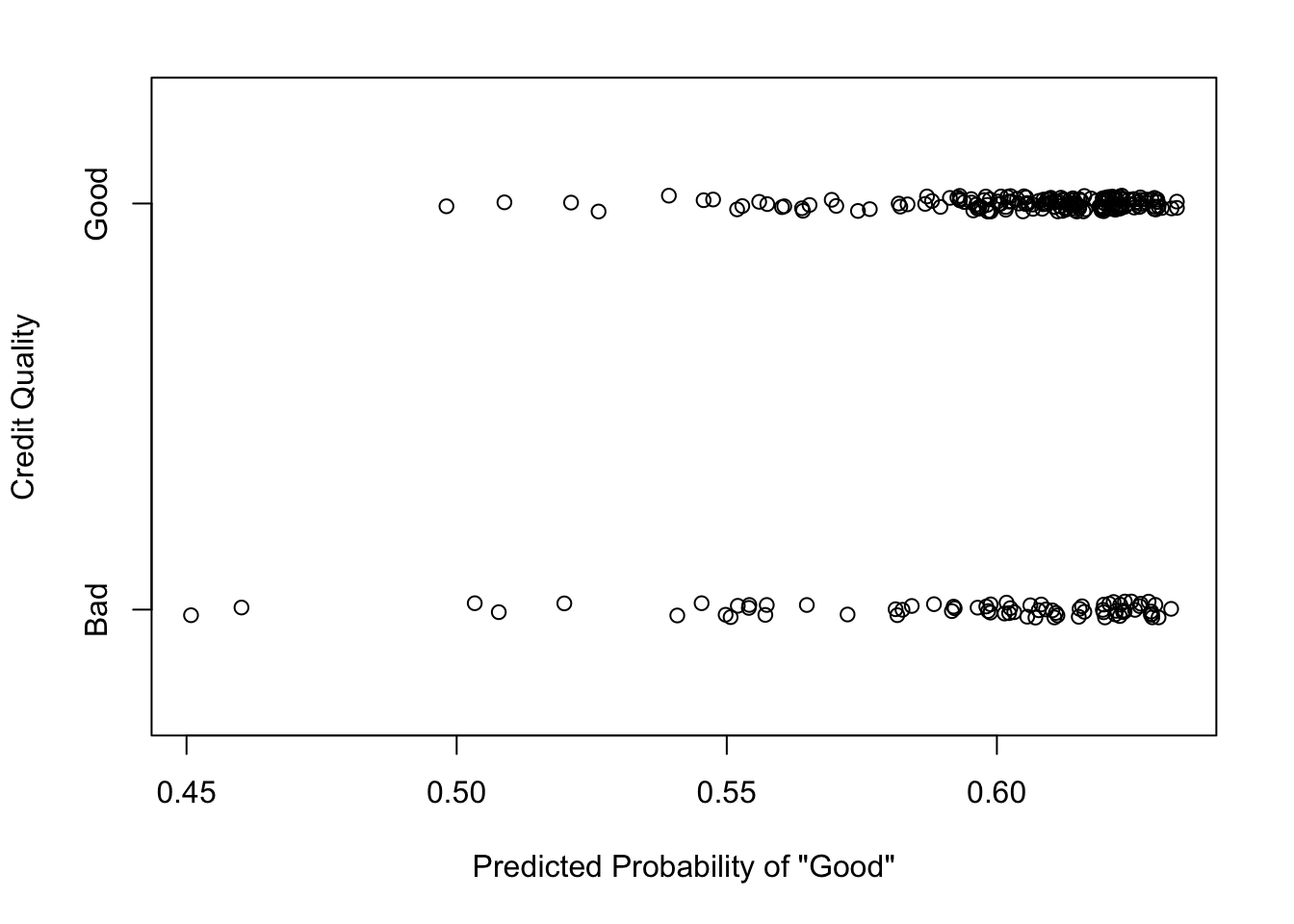
Figure 5.7: Prediction vs. Truth
Here we can see that there isn’t quite the good separation that we saw in the ideal scenario. Across the range of predicted probabilities, there are individuals with both “Good” and “Bad” credit. This suggests that the prediction algorithm that we have employed perhaps is having difficulty finding a good combination of features that can separate people with good and bad credit risk.
We can compute some summary statistics about the prediction algorithm below.
Confusion Matrix and Statistics

          Reference
Prediction Bad Good
      Bad    2    1
      Good  73  174

               Accuracy : 0.704
                 95% CI : (0.6432, 0.7599)
    No Information Rate : 0.7
    P-Value [Acc > NIR] : 0.4762

                  Kappa : 0.0289
 Mcnemar's Test P-Value : <2e-16

            Sensitivity : 0.99429
            Specificity : 0.02667
         Pos Pred Value : 0.70445
         Neg Pred Value : 0.66667
             Prevalence : 0.70000
         Detection Rate : 0.69600
   Detection Prevalence : 0.98800
      Balanced Accuracy : 0.51048

       'Positive' Class : Good
We can see that the accuracy is about 70%, which is not great for most prediction algorithms. In particular, the algorithm’s specificity is very poor, meaning that if you are a “Bad” credit risk, the probability that you will be classified as such is only about 2.6%.
7.4.0.3 Evaluation
For prediction problems, deciding on the next step after initial model fitting can depend on a few factors.
Prediction quality. Is the model’s accuracy good enough for your purposes? This depends on the ultimate goal and the risks associated with subsequent actions. For medical applications, where the outcome might be the presence of a disease, we may want to have a high sensitivity, so that if you genuinely have the disease, the algorithm will detect it. That way we can get you into treatment quickly. However, if the treatment is very painful, perhaps with many side effects, then we might actually prefer a high specificity, which would ensure that we don’t mistakenly treat someone who doesn’t have the disease. For financial applications, like the credit worthiness example used here, there may be asymmetric costs associated with mistaking good credit for bad versus mistaking bad credit for good.
Model tuning. A hallmark of prediction algorithms is their many tuning parameters. Sometimes these parameters can have large effects on prediction quality if they are changed and so it is important to be informed of the impact of tuning parameters for whatever algorithm you use. There is no prediction algorithm for which a single set of tuning parameters works well for all problems. Most likely, for the initial model fit, you will use “default” parameters, but these defaults may not be sufficient for your purposes. Fiddling with the tuning parameters may greatly change the quality of your predictions. It’s very important that you document the values of these tuning parameters so that the analysis can be reproduced in the future.
Availability of Other Data. Many prediction algorithms are quite good at exploring the structure of large and complex datasets and identifying a structure that can best predict your outcome. If you find that your model is not working well, even after some adjustment of tuning parameters, it is likely that you need additional data to improve your prediction.