9.2 Case Study: Non-diet Soda Consumption and Body Mass Index
It is probably easiest to see the principles of interpretation in action in order to learn how to apply them to your own data analysis, so we will use a case study to illustrate each of the principles.
9.2.1 Revisit the Question
The first principle is reminding yourself of your original question. This may seem like a flippant statement, but it is not uncommon for people to lose their way as they go through the process of exploratory analysis and formal modeling. This typically happens when a data analyst wanders too far off course pursuing an incidental finding that appears in the process of exploratory data analysis or formal modeling. Then the final model(s) provide an answer to another question that popped up during the analyses rather than the original question.
Reminding yourself of your question also serves to provide a framework for your interpretation. For example, your original question may have been, “For every 12-ounce can of soda drunk per day, how much greater is the average BMI among adults in the United States?” The wording of the question tells you that your original intent was to determine how much greater the BMI is among adults in the US who drink, for example, two 12-ounce cans of sodas per day on average, than among adults who drink only one 12-ounce soda per day on average. The interpretation of your analyses should yield a statement such as: For every 1 additional 12-ounce can of soda that adults in the US drink, BMI increases, on average, by X kg/m2. But it should not yield a statement such as: “For every additional ounce of soda that adults in the US drink, BMI increases, on average, by X kg/m2.”
Another way in which revisiting your question provides a framework for interpreting your results is that reminding yourself of the type of question that you asked provides an explicit framework for interpretation (See Stating and Refining the Question for a review of types of questions). For example, if your question was, “Among adults in the US, do those who drink 1 more 12-ounce serving of non-diet soda per day have a higher BMI, on average?”, this tells you that your question is an inferential question and that your goal is to understand the average effect of drinking an additional 12-ounce serving of non-diet soda per day on BMI among the US adult population. To answer this question, you may have performed an analysis using cross-sectional data collected on a sample that was representative of the US adult population, and in this case your interpretation of the result is framed in terms of what the association is between an additional 12-ounce serving of soda per day and BMI, on average in the US adult population.
Because your question was not a causal one, and therefore your analysis was not a causal analysis, the result cannot be framed in terms of what would happen if a population started consuming an additional can of soda per day. A causal question might be: “What effect does drinking an additional 12-ounce serving of non-diet soda per day have on BMI?”, and to answer this question, you might analyze data from a clinical trial that randomly assigned one group to drink an additional can of soda and the other group to drink an additional can of a placebo drink. The results from this type of question and analysis could be interpreted as what the causal effect of drinking additional 12-ounce can of soda per day would be on BMI. Because the analysis is comparing the average effect on BMI between the two groups (soda and placebo), the result would be interpreted as the average causal effect in the population.
A third purpose of revisiting your original question is that it is important to pause and consider whether your approach to answering the question could have produced a biased result. Although we covered bias to some degree in the chapter on Stating and Refining the Question, sometimes new information is acquired during the process of exploratory data analysis and/or modeling that directly affects your assessment of whether your result might be biased. Recall that bias is a systematic problem with the collection or analysis of the data that results in an incorrect answer to your question.
We will use the soda-BMI example to illustrate a simpler example of bias. Let’s assume that your overall question about the soda-BMI relationship had included an initial question, which was, “What is the mean daily non-diet soda consumption among adults in the US?” Let’s assume that your analysis indicates that in the sample you are analyzing, which is a sample of all adults in the US, the average number of 12-ounce servings of non-diet soda drunk per day is 0.5, so you infer that the average number of 12-ounce servings of soda drunk per day by adults in the US is also 0.5. Since you should always challenge your results, it is important to consider whether your analysis has an inherent bias.
So how do you do this? You start by imagining that your result is incorrect, and then think through the ways in which the data collection or analysis could have had a systematic problem that resulted in an incorrect estimate of the mean number of 12-ounce cans of non-diet soda drunk per day by adults in the US. Although this exercise of imagining that your result is wrong is discussed as an approach to assessing the potential for bias, this is a terrific way to challenge your results at every step of the analysis, whether you are assessing risk of bias, or confounding, or a technical problem with your analysis.
The thought experiment goes something like this: imagine that the true average number of 12-ounce servings of non-diet soda drunk per day by adults in the US is 2. Now imagine how the result from your analysis of the sample, which was 0.5, might be so far off from the true result: for some reason, the sample of the population that comprises your dataset is not a random sample of the population and instead has a disproportionate number of people who do not drink any non-diet soda, which brings down the estimated mean number of 12 ounces of servings of non-diet soda consumed per day. You might also imagine that if your sample result had been 4, which is much higher than the true amount drunk per day by adults in the US, that your sample has a disproportionate number of people who have high consumption of non-diet soda so that the estimate generated from your analyses is higher than the true value. So how can you gauge whether your sample is non-random?
To figure out if your sample is a non-random sample of the target population, think about what could have happened to attract more people who don’t consume non-diet soda (or more people who consume a lot of it) to be included in the sample. Perhaps the study advertised for participation in a fitness magazine, and fitness magazine readers are less likely to drink non-diet soda. Or perhaps the data were collected by an internet survey and internet survey respondents are less likely to drink non-diet soda. Or perhaps the survey captured information about non-diet soda consumption by providing a list of non-diet sodas and asking survey respondents to indicate which ones they had consumed, but the survey omitted Mountain Dew and Cherry Coke, so that those people who drink mostly these non-diet sodas were classified as not consuming non-diet soda (or consuming less of it than they actually do consume). And so on.
Although we illustrated the simplest scenario for bias, which occurs when estimating a prevalence or a mean, you of course can get a biased result for an estimate of a relationship between two variables as well. For example, the survey methods could unintentionally oversample people who both don’t consume non-diet soda and have a high BMI (such as people with type 2 diabetes), so that the result would indicate (incorrectly) that consuming non-diet soda is not associated with having a higher BMI. The point is that pausing to perform a deliberate thought experiment about sources of bias is critically important as it is really the only way to assess the potential for a biased result. This thought experiment should also be conducted when you are stating and refining your question and also as you are conducting exploratory analyses and modeling.
9.2.2 Start with the primary model and assess the directionality, magnitude, and uncertainty of the result
The second principle is to start with a single model and focus on the full continuum of the result, including its directionality and magnitude, and the degree of certainty (or uncertainty) there is about whether the result from the sample you analyzed reflects the true result for the overall population. A great deal of information that is required for interpreting your results will be missed if you zoom in on a single feature of your result (such as the p-value), so that you either ignore or gloss over other important information provided by the model. Although your interpretation isn’t complete until you consider the results in totality, it is often most helpful to first focus on interpreting the results of the model that you believe best answers your question and reflects (or “fits”) your data, which is your primary model (See Formal Modeling). Don’t spend a lot of time worrying about which single model to start with, because in the end you will consider all of your results and this initial interpretation exercise serves to orient you and provide a framework for your final interpretation.
9.2.2.1 Directionality
Building on the soda-BMI example, take a look at sample dataset below with a fitted model overlaid.
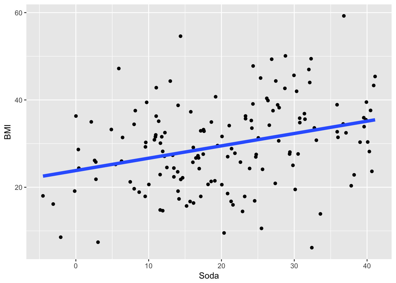
Figure 9.1: Sample Data for BMI-soda Example
We will focus on what the model tells us about the directionality of the relationship between soda consumption and BMI, the magnitude of the relationship, and the uncertainty of the relationship, or how likely the model’s depiction of the relationship between non-diet soda consumption and BMI is real vs. just a reflection of random variation you’d expect when sampling from a larger population.
The model indicates that the directionality of the relationship is positive, meaning that as non-diet soda consumption increases, BMI increases. The other potential results could have been a negative directionality, or no directionality (a value of approximately 0). Does the positive directionality of the result match your expectations that have been developed from the exploratory data analysis? If so, you’re in good shape and can move onto the next interpretation activity. If not, there are a couple of possible explanations. First your expectations may not be correct because either the exploratory analysis was done incorrectly or your interpretation of the exploratory analyses was not correct. Second, the exploratory analysis and your interpretation of it may be correct, but the formal modeling may have been done incorrectly. Notice that with this process, you are once again applying the epicycle of data analysis.
9.2.2.2 Magnitude
Once you have identified and addressed any discrepancies between your expectations and interpretation of the directionality of the relationship, the next step is to consider the magnitude of the relationship. Because the model is a linear regression, you can see that the slope of the relationship, reflected by the beta coefficient, is 0.28. Interpreting the slope requires knowing the units of the “soda” variable. If the units are 12-ounce cans of soda per day, then the interpretation of this slope is that BMI increases by 0.28 kg/m2 per additional 12-ounce can of non-diet soda that is consumed per day. However, the units are in ounces of soda, so the interpretation of your model is that BMI increases by 0.28 kg/m2 for each additional ounce of non-diet soda that is consumed per day.
Although you’re comfortable that you understand the units of your soda variable correctly and have the correct interpretation of the model, you still don’t quite have the answer to your question, which was framed in terms of the association of each additional 12-ounce can of soda and BMI, not each additional ounce of non-diet soda. So you’ll need to convert the 0.28 slope so that it pertains to a 12-ounce, rather than 1 ounce, increase in soda consumption. Because the model is a linear model, you can simply multiply the slope, or beta coefficient, by 12 to get 3.36, which tells you that each additional 12-ounce can of soda consumed per day is associated with a BMI that is 3.36 kg/m2 higher.
The other option of course is to create a new soda variable whose unit is 12 ounces rather than 1 ounce, but multiplying the slope is a simple mathematical operation and is much more efficient. Here again you should have had some expectations, based on the exploratory data analysis you did, about the magnitude of the relationship between non-diet soda consumption and BMI, so you should determine if your interpretation of the magnitude of the relationship matches your expectations. If not, you’ll need to determine whether your expectations were incorrect or whether your interpretation was incorrect and act accordingly to match expectations and the result of your interpretation.
Another important consideration about the magnitude of the relationship is whether it is meaningful. For example, a 0.01 increase in BMI for every additional 20 ounces consumed per day is probably not particularly meaningful as a large amount of soda is associated with a very small increase in BMI. On the other hand, if there were a 0.28 kg/m2 increase in BMI for every 1 ounce increase in soda consumption, this would in fact be quite meaningful. Because you know BMI generally ranges from the high teens to the 30’s, a change of 0.01 kg/m2 is small, but a change of 0.28 kg/m2 could be meaningful.
When taken in the context of the kinds of volumes of soda people might consume, a 0.01 kg/m2 for each 20 ounce increase in soda consumption is small since people are (hopefully) not drinking 10 twenty ounce servings per day, which is how much someone would need to drink in order to observe even a 0.1 kg/m2 increase in BMI. On the other hand a 0.28 kg/m2 increase in BMI for every additional ounce of soda would add up quickly for people who consumed an extra 20 ounce non-diet soda per day - this would equate to an expected increase in BMI of 5.6 kg/m2. A key part of interpreting the magnitude of the result, then, is understanding how the magnitude of the result compares to what you know about this type of information in the population you’re interested in.
9.2.2.3 Uncertainty
Now that you have a handle on what the model says about the directionality and magnitude of the relationship between non-diet soda consumption and BMI, the next step it to consider what the degree of uncertainty is for your answer. Recall that your model has been constructed to fit data collected from a sample of the overall population and that you are using this model to understand how non-diet soda consumption is related to BMI in the overall population of adults in the US.
Let’s get back to our soda-BMI example, which does involve using the results that are obtained on the sample to make inferences about what the true soda-BMI relationship is in the overall population of adults in the US. Let’s imagine that the result from your analysis of the sample data indicates that within your sample, people who drink an additional ounce of non-diet soda per day have a BMI that is 0.28 kg/m2 greater than those who drink an ounce less per day. However, how do you know whether this result is simply the “noise” of random sampling or whether it is a close approximation of the true relationship among the overall population?
To assess whether the result from the sample is simply random “noise”, we use measures of uncertainty. Although some might expect that all random samples serve as excellent surrogates for the overall population, this is not true. To illustrate this idea using a simple example, imagine that the prevalence of females in the overall US adult population is 51%, and you draw a random sample of 100 adults. This sample may have 45% females. Imagine that you draw a new sample of 100 adults and your sample has 53% females. You could draw many samples like this and even draw samples of 35% or 70% females. The probability of drawing a sample with a prevalence of females that is this different from the overall population prevalence of females is very small, while the probability of drawing a sample that has close to 51% females is much higher.
It is this concept—the probability that your sample reflects the answer for the overall population varies depending on how close (or far) your sample result is to the true result for the overall population—that is the bedrock of the concept of uncertainty. Because we don’t know what the answer is for the overall population (that’s why we’re doing the analysis in the first place!), it’s impossible to express uncertainty in terms of how likely or unlikely it is that your sample result reflects the overall population. So there are other approaches to measuring uncertainty that rely on this general concept, and we will discuss two common approaches below.
One tool that provides a more continuous measure of uncertainty is the confidence interval. A confidence interval is a range of values that contains your sample result and you have some amount of confidence that it also contains the true result for the overall population. Most often statistical modeling software provides 95% confidence intervals, so that if the 95% CI for the sample estimate of 0.28 kg/m2 from above is 0.15–0.42 kg/m2, the approximate interpretation is that you can be 95% confident that the true result for the overall population is somewhere between 0.15 and 0.42 kg/m2.
A more precise definition of the 95% confidence interval would be that over repeated samples, if we were to conduct this experiment many times (each time collecting a dataset of the same size) then a confidence interval constructed in this manner would cover the truth 95% of the time. It’s important to realize that because the confidence interval is constructed from the data, the interval itself is random. Therefore, if we were to collect new data, the interval we’d construct would be slightly different. However, the truth, meaning the population value of the parameter, would always remain the same.
Another tool for measuring uncertainty is, of course, the p-value, which simply is the probability of getting the sample result of 0.28 kg/m2 (or more extreme) when the true relationship between non-diet soda consumption and BMI in the overall population is 0. Although the p-value is a continuous measure of uncertainty, many people consider a p-value of <0.05, which indicates that there is a less than 5% probability of observing the sample result (or a more extreme result) when there is no relationship in the overall population, as “statistically significant”. This cutpoint is arbitrary and tells us very little about the degree of uncertainty or about where the true answer for the overall population lies. Focusing primarily on the p-value is a risky approach to interpreting uncertainty because it can lead to ignoring more important information needed for thoughtful and accurate interpretation of your results.
The CI is more helpful than the p-value, because it gives a range, which provides some quantitative estimate about what the actual overall population result is likely to be, and it also provides a way to express how certain it is that the range contains the overall population result.
Let’s walk through how the p-value vs. 95% CI would be used to interpret uncertainty about the result from the soda-BMI analysis. Let’s say that our result was that BMI was 0.28 kg/m2 higher on average among our sample who drank one ounce more of non-diet soda per day and that the p-value associated with this result was 0.03. Using the p-value as a tool for measuring uncertainty and setting a threshold of statistical significance at 0.05, we would interpret the uncertainty as follows: there is a less than 5% chance that we would get this result (0.28) or something more extreme if the true population value was 0 (or in other words, that there was really not an association between soda consumption and BMI in the overall population).
Now let’s go through the same exercise with the 95% CI. The 95% CI for this analysis is 0.15–0.42. Using the CI as the tool for interpreting uncertainty, we could say that we are 95% confident that the true relationship between soda consumption and BMI in the adult US population lies somewhere between a 0.15 and 0.42 kg/m2 increase in BMI on average per additional ounce of non-diet soda that is consumed. Using this latter approach tells us something about the range of possible effects of soda on BMI and also tells us that it is very unlikely that soda has no association with BMI in the overall population of adults in the US. Using the p-value as the measure of uncertainty, on the other hand, implies that we have only two choices in terms of interpreting the result: either there is a good amount of uncertainty about it so we must conclude that there is no relationship between soda consumption and BMI, or there is very little uncertainty about the result so we must conclude that there is a relationship between soda consumption and BMI. Using the p-value constrains us in a way that does not reflect the process of weighing the strength of the evidence in favor (or against) a hypothesis.
Another point about uncertainty is that we have discussed assessing uncertainty through more classical statistical approaches, which are based on the Frequentist paradigm, which is the most common approach. The Bayesian framework is an alternate approach in which you update your prior beliefs based on the evidence provided by the analysis. In practice, the Frequentist approach we discussed above is more commonly used, and in real-world setting rarely leads to conclusions that would be different from those obtained by using a Bayesian approach.
One important caveat is that sometimes evaluating uncertainty is not necessary because some types of analyses are not intended to make inferences about a larger overall population. If, for example, you wanted to understand the relationship between age and dollars spent per month on your company’s products, you may have all of the data on the entire, or “overall” population you are interested in, which is your company’s customers. In this case you do not have to rely on a sample, because your company collects data about the age and purchases of ALL of their customers. In this case, you would not need to consider the uncertainty that your result reflects the truth for the overall population because your analysis result is the truth for your overall population.
9.2.3 Develop an overall interpretation by considering the totality of your analyses and external information
Now that you have dedicated a good amount of effort interpreting the results of your primary model, the next step is to develop an overall interpretation of your results by considering both the totality of your analyses and information external to your analyses. The interpretation of the results from your primary model serves to set the expectation for your overall interpretation when you consider all of your analyses. Building on the soda-BMI example, let’s assume that your interpretation of your primary model is that BMI is 0.28 kg/m2 higher on average among adults in the US who consume an average one additional ounce of soda per day. Recall that this primary model was constructed after gathering information through exploratory analyses and that you may have refined this model when you were going through the process of interpreting its results by evaluating the directionality, magnitude and uncertainty of the model’s results.
As discussed in the Formal Modeling chapter, there is not one single model that alone provides the answer to your question. Instead, there are additional models that serve to challenge the result obtained in the primary model. A common type of secondary model is the model which is constructed to determine how sensitive the results in your primary model are to changes in the data. A classic example is removing outliers to assess the degree to which your primary model result changes. If the primary model results were largely driven by a handful of, for example, very high soda consumers, this finding would suggest that there may not be a linear relationship between soda consumption and BMI and that instead soda consumption may only influence BMI among those who have very high consumption of soda. This finding should lead to a revision of your primary model.
A second example is evaluating the effect of potential confounders on the results from the primary model. Although the primary model should already contain key confounders, there are typically additional potential confounders that should be assessed. In the soda-BMI example, you may construct a secondary model that includes income because you realize that it is possible that the relationship you observe in your primary model could be explained entirely by socioeconomic status: people of higher socioeconomic status might drink less non-diet soda and also have lower BMIs, but it is not because they drink less soda that this is the case. Instead, it is some other factor associated with socioeconomic status that has the effect on BMI. So you can run a secondary model in which income is added to the primary model to determine if this is the case. Although there are other examples of uses of secondary models, these are two common examples.
So how do you interpret how these secondary model results affect your primary result? You can fall back on the paradigm of: directionality, magnitude, and uncertainty. When you added income to the soda-BMI model, did income change the directionality of your estimated relationship between soda and BMI from the primary model - either to a negative association or no association? If it did, that would be a dramatic change and suggest that either something is not right with your data (such as with the income variable) or that the association between soda consumption and BMI is entirely explained by income.
Let’s assume that adding income did not change the directionality and suppose that it changed the magnitude so that the primary model’s estimate of 0.28 kg/m2 decreased to 0.12kg/m2. The magnitude of the relationship between soda and BMI was reduced by 57%, so this would be interpreted as income explaining a little more than half, but not all, of the relationship between soda consumption and BMI.
Now you move on to uncertainty. The 95% CI for the estimate with the model that includes income is 0.01–0.23, so that we can be 95% confident that the true relationship between soda and BMI in the adult US population, independent of income, lies somewhere in this range. What if the 95% CI for the estimate were -0.02–0.26, but the estimate was still 0.12 kg/m2? Even though the CI now includes 0, the result from the primary model, 0.12, did not change, indicating that income does not appear to explain any of the association between soda consumption and BMI, but that it did increase the uncertainty of the result. One reason that the addition of income to the model could have increased the uncertainty is that some people in the sample were missing income data so that the sample size was reduced. Checking your n’s will help you determine if this is the case.
It’s also important to consider your overall results in the context of external information. External information is both general knowledge that you or your team members have about the topic, results from similar analyses, and information about the target population. One example discussed above is that having a sense of what typical and plausible volumes of soda consumption are among adults in the US is helpful for understanding if the magnitude of the effect of soda consumption on BMI is meaningful. It may also be helpful to know what percent of the adult population in the US drinks non-diet soda and the prevalence of obesity to understand the size of the population for whom your results might be pertinent.
One interesting example of how important it is to think about the size of the population that may be affected is air pollution. For associations between outdoor air pollution and critical health outcomes such as cardiovascular events (stroke, heart attack), the magnitude of the effect is small, but because air pollution affects hundreds of millions of people in the US, the numbers of cardiovascular events attributable to pollution is quite high.
In addition, you probably are not the first person to try and answer this question or related questions. Others may have done an analysis to answer the question in another population (adolescents, for example) or to answer a related, but different question, such as: “what is the relationship between non-diet soda consumption and blood sugar levels?” Understanding how your results fit into the context of the body of knowledge about the topic helps you and others assess whether there is an overall story or pattern emerging across all sources of knowledge that point to non-diet soda consumption being linked to high blood sugar, insulin resistance, BMI, and type 2 diabetes. On the other hand, if the results of your analysis differ from the external knowledge base, that is important too. Although most of the time when the results are so strikingly different from external knowledge, there is an explanation such as an error or differences in methods of data collection or population studied, sometimes a distinctly different finding is a truly novel insight.
9.2.4 Implications
Now that you’ve interpreted your results and have conclusions in hand, you’ll want to think about the implications of your conclusions. After all, the point of doing an analysis is usually to inform a decision or to take an action. Sometimes the implications are straightforward, but other times the implications take some thought. An example of a straightforward implication is if you performed an analysis to determine if purchasing ads increased sales, and if so, did the investment in ads result in a net profit. You may learn that either there was a net profit or not, and if there were a net profit, this finding would support continuing the ads.
A more complicated example is the soda-BMI example we’ve used throughout this chapter. If soda consumption turned out to be associated with higher BMI, with a 20 ounce additional serving per day associated with a 0.28 kg/m2 greater BMI, this finding would imply that if you could reduce soda consumption, you could reduce the average BMI of the overall population. Since your analysis wasn’t a causal one, though, and you only demonstrated an association, you may want to perform a study in which you randomly assign people to either replacing one of the 20 ounce sodas they drink each day with diet soda or to not replacing their non-diet soda. In a public health setting, though, your team may decide that this association is sufficient evidence to launch a public health campaign to reduce soda consumption, and that you do not need additional data from a clinical trial. Instead, you may plan to track the population’s BMI during and after the public health campaign as a means of estimating the public health effect of reducing non-diet soda consumption. The take-home point here is that the action that results from the implications often depends on the mission of the organization that requested the analysis.