7.3 Associational Analyses
Associational analyses are ones where we are looking at an association between two or more features in the presence of other potentially confounding factors. There are three classes of variables that are important to think about in an associational analysis.
Outcome. The outcome is the feature of your dataset that is thought to change along with your key predictor. Even if you are not asking a causal or mechanistic question, so you don’t necessarily believe that the outcome responds to changes in the key predictor, an outcome still needs to be defined for most formal modeling approaches.
Key predictor. Often for associational analyses there is one key predictor of interest (there may be a few of them). We want to know how the outcome changes with this key predictor. However, our understanding of that relationship may be challenged by the presence of potential confounders.
Potential confounders. This is a large class of predictors that are both related to the key predictor and the outcome. It’s important to have a good understanding what these are and whether they are available in your dataset. If a key confounder is not available in the dataset, sometimes there will be a proxy that is related to that key confounder that can be substituted instead.
Once you have identified these three classes of variables in your dataset, you can start to think about formal modeling in an associational setting.
The basic form of a model in an associational analysis will be
\[ y = \alpha + \beta x + \gamma z + \varepsilon \]
where
- \(y\) is the outcome
- \(x\) is the key predictor
- \(z\) is a potential confounder
- \(\varepsilon\) is independent random error
- \(\alpha\) is the intercept, i.e. the value \(y\) when \(x=0\) and \(z=0\)
- \(\beta\) is the change in \(y\) associated with a 1-unit increase \(x\), adjusting for \(z\)
- \(\gamma\) is the change in \(y\) associated with a 1-unit increase in \(z\), adjusting for \(x\)
This is a linear model, and our primary interest is in estimating the coefficient \(\beta\), which quantifies the relationship between the key predictor \(x\) and the outcome \(y\).
Even though we will have to estimate \(\alpha\) and \(\gamma\) as part of the process of estimating \(\beta\), we do not really care about the values of those \(\alpha\) and \(\gamma\). In the statistical literature, coefficients like \(\alpha\) and \(\gamma\) are sometimes referred to as nuisance parameters because we have to use the data to estimate them to complete the model specification, but we do not actually care about their value.
The model shown above could be thought of as the primary model. There is a key predictor and one confounder in the model where it is perhaps well known that you should adjust for that confounder. This model may produce sensible results and follows what is generally known in the area.
7.3.1 Example: Online advertising campaign
Suppose we are selling a new product on the web and we are interested in whether buying advertisements on Facebook helps to increase the sales of that product. To start, we might initiate a 1-week pilot advertising campaign on Facebook and gauge the success of that campaign. If it were successful, we might continue to buy ads for the product.
One simple approach might be to track daily sales before, during, and after the advertising campaign (note that there are more precise ways to do this with tracking URLs and Google Analytics, but let’s leave that aside for now). Put simply, if the campaign were a week long, we could look at the week before, the week during, and the week after to see if there were any shifts in the daily sales.
7.3.1.1 Expectations
In an ideal world, the data might look something like this.
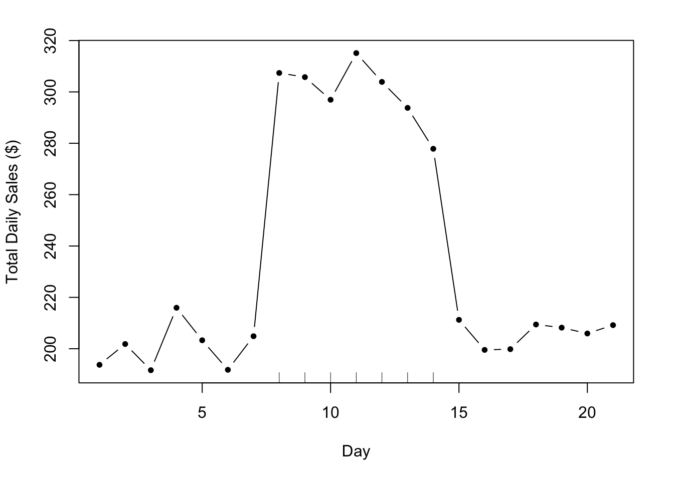
Figure 7.1: Hypothetical Advertising Campaign
The tick marks on the x-axis indicate the period when the campaign was active. In this case, it’s pretty obvious what effect the advertising campaign had on sales. Using just your eyes, it’s possible to tell that the ad campaign added about $100 per day to total daily sales. Your primary model might look something like
\[ y = \alpha + \beta x + \varepsilon \]
where \(y\) is total daily sales and \(x\) is and indicator of whether a given day fell during the ad campaign or not. The hypothetical data for the plot above might look as follows.
      sales campaign day
1  193.7355        0   1
2  201.8364        0   2
3  191.6437        0   3
4  215.9528        0   4
5  203.2951        0   5
6  191.7953        0   6
7  204.8743        0   7
8  307.3832        1   8
9  305.7578        1   9
10 296.9461        1  10
11 315.1178        1  11
12 303.8984        1  12
13 293.7876        1  13
14 277.8530        1  14
15 211.2493        0  15
16 199.5507        0  16
17 199.8381        0  17
18 209.4384        0  18
19 208.2122        0  19
20 205.9390        0  20
21 209.1898        0  21
Given this data and the primary model above, we’d estimate \(\beta\) to be $96.78, which is not far off from our original guess of $100.
Setting Expectations. The discussion of this ideal scenario is important not because it’s at all likely to occur, but rather because it instructs on what we would expect to see if the world operated according to a simpler framework and how we would analyze the data under those expectations.
7.3.1.2 More realistic data
Unfortunately, we rarely see data like the plot above. In reality, the effect sizes tend to be smaller, the noise tends to be higher, and there tend to be other factors at play. Typically, the data will look something like this.
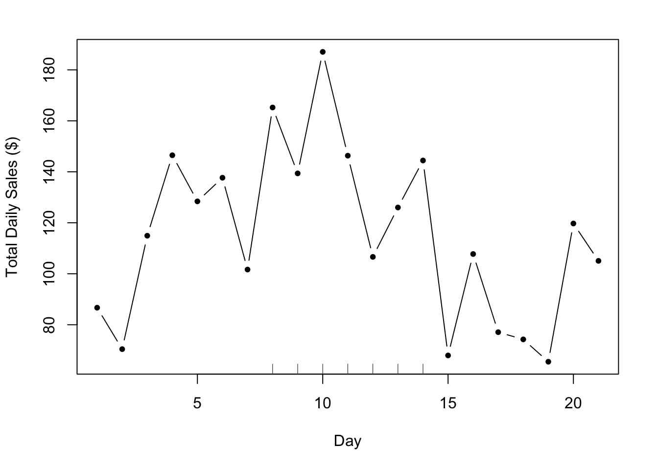
Figure 5.2: More Realistic Daily Sales Data
While it does appear that there is an increase in sales during the period of the ad campaign (indicated by the tick marks again), it’s a bit difficult to argue that the increased sales are caused by the campaign. Indeed, in the days before the campaign starts, there appears to be a slight increase in sales. Is that by chance or are there other trends going on in the background? It’s possible that there is a smooth background trend so that daily sales tend to go up and down throughout the month. Hence, even without the ad campaign in place, it’s possible we would have seen an increase in sales anyway. The question now is whether the ad campaign increased daily sales on top of this existing background trend.
Let’s take our primary model, which just includes the outcome and the indicator of our ad campaign as a key predictor. Using that model we estimate \(\beta\), the increase in daily sales due to the ad campaign, to be $44.75.
However, suppose we incorporated a background trend into our model, so instead of our primary model, we fit the following.
\[ y = \alpha + \beta x + \gamma_1 t + \gamma_2 t^2 + \varepsilon \]
where \(t\) now indicates the day number (i.e. \(1,2,\dots,21\)). What we have done is add a quadratic function of \(t\) to the model to allow for some curvature in the trend (as opposed to a linear function that would only allow for a strictly increasing or decreasing pattern). Using this model we estimate \(\beta\) to be $39.86, which is somewhat less than what the primary model estimated for \(\beta\).
We can fit one final model, which allows for an even more flexible background trend–we use a 4th order polynomial to represent that trend. Although we might find our quadratic model to be sufficiently complex, the purpose of this last model is to just push the envelope a little bit to see how things change in more extreme circumstances. This model gives us an estimate of \(\beta\) of $49.1, which is in fact larger than the estimate from our primary model.
At this point we have a primary model and two secondary models, which give somewhat different estimates of the association between our ad campaign and daily total sales.
| Model | Features | Estimate for \(\beta\) |
|---|---|---|
| Model 1 (primary) | No confounders | $44.75 |
| Model 2 (secondary) | Quadratic time trend | $39.86 |
| Model 3 (secondary) | 4th order time trend | $49.1 |
7.3.1.3 Evaluation
Determining where to go from here may depend on factors outside of the dataset. Some typical considerations are
Effect size. The three models present a range of estimates from $39.86 to $49.1. Is this a large range? It’s possible that for your organization a range of this magnitude is not large enough to really make a difference and so all of the models might be considered equivalent. Or you might consider these 3 estimates to be significantly different from each other, in which case you might put more weight on one model over another. Another factor might be the cost of the advertising campaign, in which case you would be interested in the return on your investment in the ads. An increase in $39.86 per day might be worth it if the total ad cost were $10 per day, but maybe not if the cost were $20 per day. Then, you might need the increase in sales to be higher to make the campaign worthwhile. The point here is that there’s some evidence from your formal model that the ad campaign might only increase your total daily sales by 39.86, however, other evidence says it might be higher. The question is whether you think it is worth the risk to buy more ads, given the range of possibilities, or whether you think that even at the higher end, it’s probably not worth it.
Plausibility. Although you may fit a series of models for the purposes of challenging your primary model, it may be the case that some models are more plausible than others, in terms of being close to whatever the “truth” about the population is. Here, the model with a quadratic trend seems plausible because it is capable of capturing a possible rise-and-fall pattern in the data, if one were present. The model with the 4th order polynomial is similarly capable of capturing this pattern, but seems overly complex for characterizing a simple pattern like that. Whether a model could be considered more or less plausible will depend on your knowledge of the subject matter and your ability to map real-world events to the mathematical formulation of the model. You may need to consult with other experts in this area to assess the plausibility of various models.
Parsimony. In the case where the different models all tell the same story (i.e. the estimates are \(\beta\) are close enough together to be considered “the same”), it’s often preferable to choose the model that is simplest. There are two reasons for this. First, with a simpler model it can be easier to tell a story about what is going on in the data via the various parameters in the model. For example, it’s easier to explain a linear trend than it is to explain an exponential trend. Second, simpler models, from a statistical perspective, are more “efficient”, so that they make better use of the data per parameter that is being estimated. Complexity in a statistical model generally refers to the number of parameters in the model–in this example the primary model has 2 parameters, whereas the most complex model has 6 parameters. If no model produces better results than another, we might prefer a model that only contains 2 parameters because it is simpler to describe and is more parsimonious. If the primary and secondary models produce significant differences, then might choose a parsimonious model over a more complex model, but not if the more complex model tells a more compelling story.