8.2 Inferring an Association
The first approach we will take will be to ask, “Is there an association between daily 24-hour average PM10 levels and daily mortality?” This is an inferential question and we are attempting to estimate an association. In addition, for this question, we know there are a number of potential confounders that we will have to deal with.
Let’s take a look at the bivariate association between PM10 and mortality. Here is a scatterplot of the two variables.
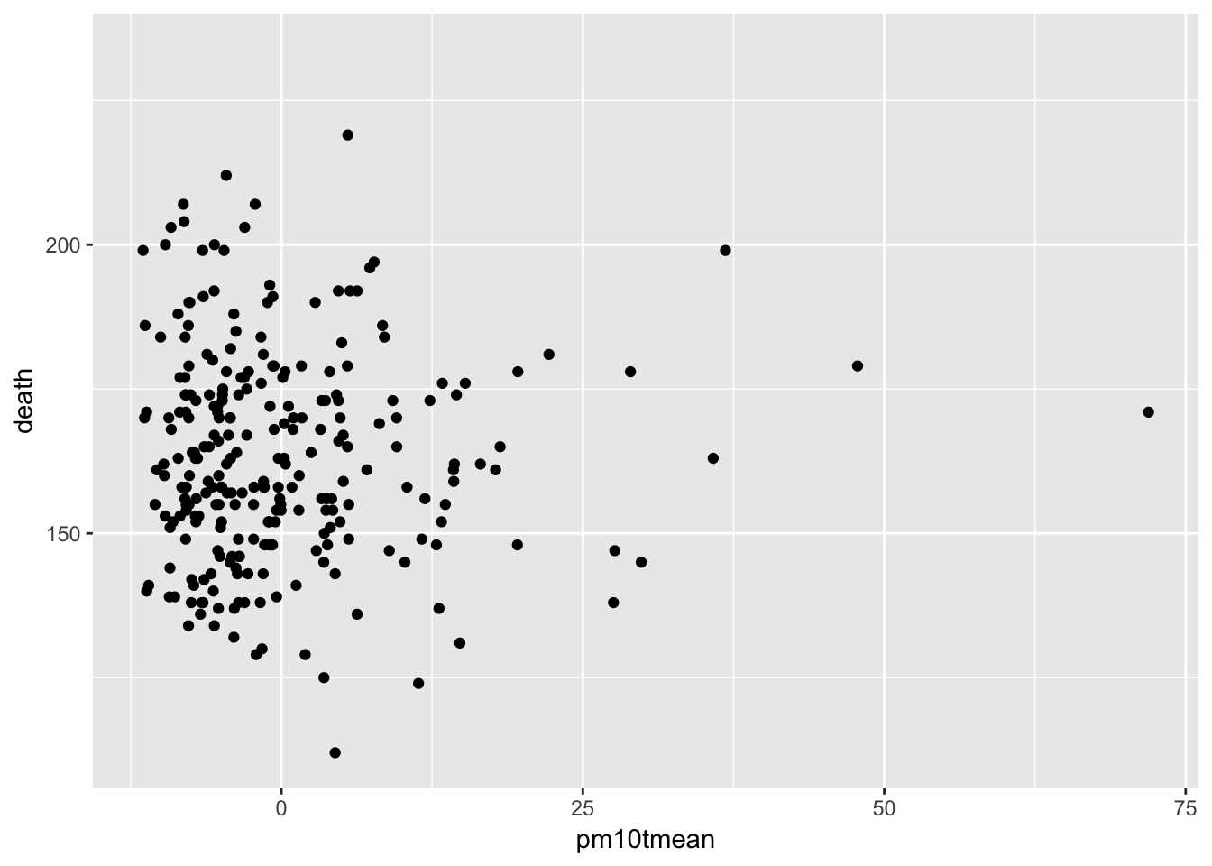
Figure 5.2: PM10 and Mortality in New York City
There doesn’t appear to be much going on there, and a simple linear regression model of the log of daily mortality and PM10 seems to confirm that.
                 Estimate   Std. Error      t value  Pr(>|t|)
(Intercept) 5.08884308354 0.0069353779 733.75138151 0.0000000
pm10tmean   0.00004033446 0.0006913941   0.05833786 0.9535247
In the table of coefficients above, the coefficient for pm10tmean is quite small and its standard error is relatively large. Effectively, this estimate of the association is zero.
However, we know quite a bit about both PM10 and daily mortality, and one thing we do know is that season plays a large role in both variables. In particular, we know that mortality tends to be higher in the winter and lower in the summer. PM10 tends to show the reverse pattern, being higher in the summer and lower in the winter. Because season is related to both PM10 and mortality, it is a good candidate for a confounder and it would make sense to adjust for it in the model.
Here are the results for a second model, which includes both PM10 and season. Season is included as an indicator variable with 4 levels.
                Estimate   Std. Error    t value     Pr(>|t|)
(Intercept)  5.166484285 0.0112629532 458.714886 0.000000e+00
seasonQ2    -0.109271301 0.0166902948  -6.546996 3.209291e-10
seasonQ3    -0.155503242 0.0169729148  -9.161847 1.736346e-17
seasonQ4    -0.060317619 0.0167189714  -3.607735 3.716291e-04
pm10tmean    0.001499111 0.0006156902   2.434847 1.558453e-02
Notice now that the pm10tmean coefficient is quite a bit larger than before and its t value is large, suggesting a strong association. How is this possible?
It turns out that we have a classic example of Simpson’s Paradox here. The overall relationship between P10 and mortality is null, but when we account for the seasonal variation in both mortality and PM10, the association is positive. The surprising result comes from the opposite ways in which season is related to mortality and PM10.
So far we have accounted for season, but there are other potential confounders. In particular, weather variables, such as temperature and dew point temperature, are also both related to PM10 formation and mortality.
In the following model we include temperature (tmpd) and dew point temperature (dptp). We also include the date variable in case there are any long-term trends that need to be accounted for.
                  Estimate    Std. Error    t value     Pr(>|t|)
(Intercept)  5.62066568788 0.16471183741 34.1242365 1.851690e-96
date        -0.00002984198 0.00001315212 -2.2689856 2.411521e-02
seasonQ2    -0.05805970053 0.02299356287 -2.5250415 1.218288e-02
seasonQ3    -0.07655519887 0.02904104658 -2.6361033 8.906912e-03
seasonQ4    -0.03154694305 0.01832712585 -1.7213252 8.641910e-02
tmpd        -0.00295931276 0.00128835065 -2.2969777 2.244054e-02
dptp         0.00068342228 0.00103489541  0.6603781 5.096144e-01
pm10tmean    0.00237049992 0.00065856022  3.5995189 3.837886e-04
Notice that the pm10tmean coefficient is even bigger than it was in the previous model. There appears to still be an association between PM10 and mortality. The effect size is small, but we will discuss that later.
Finally, another class of potential confounders includes other pollutants. Before we place blame on PM10 as a harmful pollutant, it’s important that we examine whether there might be another pollutant that can explain what we’re observing. NO2 is a good candidate because it shares some of the same sources as PM10 and is known to be related to mortality. Let’s see what happens when we include that in the model.
                  Estimate    Std. Error    t value     Pr(>|t|)
(Intercept)  5.61378604085 0.16440280471 34.1465345 2.548704e-96
date        -0.00002973484 0.00001312231 -2.2659756 2.430503e-02
seasonQ2    -0.05143935218 0.02338034983 -2.2001105 2.871069e-02
seasonQ3    -0.06569205605 0.02990520457 -2.1966764 2.895825e-02
seasonQ4    -0.02750381423 0.01849165119 -1.4873639 1.381739e-01
tmpd        -0.00296833498 0.00128542535 -2.3092239 2.174371e-02
dptp         0.00070306996 0.00103262057  0.6808599 4.965877e-01
no2tmean     0.00126556418 0.00086229169  1.4676753 1.434444e-01
pm10tmean    0.00174189857 0.00078432327  2.2208937 2.725117e-02
Notice in the table of coefficients that the no2tmean coefficient is similar in magnitude to the pm10tmean coefficient, although its t value is not as large. The pm10tmean coefficient appears to be statistically significant, but it is somewhat smaller in magnitude now.
Below is a plot of the PM10 coefficient from all four of the models that we tried.
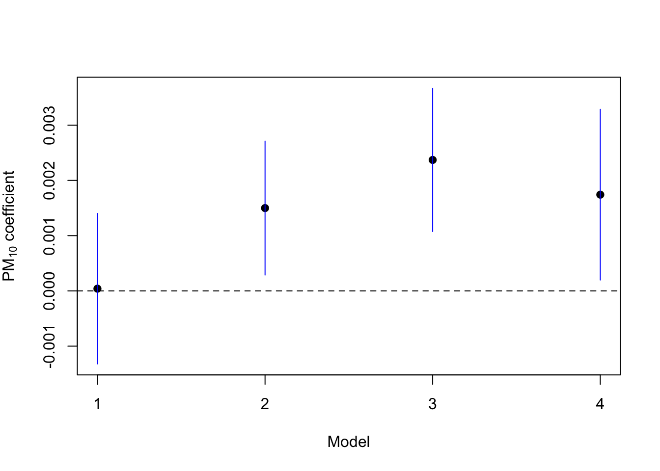
Figure 5.5: Association Between PM10 and Mortality Under Different Models
With the exception of Model 1, which did not account for any potential confounders, there appears to be a positive association between PM10 and mortality across Models 2–4. What this means and what we should do about it depends on what our ultimate goal is and we do not discuss that in detail here. It’s notable that the effect size is generally small, especially compared to some of the other predictors in the model. However, it’s also worth noting that presumably, everyone in New York City breathes, and so a small effect could have a large impact.