12.10 Lab: R Code

12.10.1 Clustered Standard Errors

Further below we use clustered standard errors for some estimations (clustering according to ethnic group and district). Sometimes this is slightly more complicated in R than in Stata (see Arai 2015; Esarey 2016). Here we use two functions based on Arai (2015) but in future you may rely on the clusterSEs package by Esarey and Menger (2016) (see ?clusterSEs for instructions on how to use it).

# One-way cluster function (Arai 2015)
clx <-
  function(fm, dfcw, cluster){
  library(sandwich)
  library(lmtest)
  M <- length(unique(cluster))
  N <- length(cluster)
  dfc <- (M/(M-1))*((N-1)/(N-fm$rank))
  u <- apply(estfun(fm),2,
  function(x) tapply(x, cluster, sum))
  vcovCL <- dfc*sandwich(fm, meat=crossprod(u)/N)*dfcw
  coeftest(fm, vcovCL) }


# Two-way cluster function (Arai 2015)
mclx <-
  function(fm, dfcw, cluster1, cluster2){
  library(sandwich)
  library(lmtest)
  cluster12 = paste(cluster1,cluster2, sep="")
  M1 <- length(unique(cluster1))
  M2 <- length(unique(cluster2))
  M12 <- length(unique(cluster12))
  N <- length(cluster1)
  K <- fm$rank
  dfc1 <- (M1/(M1-1))*((N-1)/(N-K))
  dfc2 <- (M2/(M2-1))*((N-1)/(N-K))
  dfc12 <- (M12/(M12-1))*((N-1)/(N-K))
  u1 <- apply(estfun(fm), 2,
  function(x) tapply(x, cluster1, sum))
  u2 <- apply(estfun(fm), 2,
  function(x) tapply(x, cluster2, sum))
  u12 <- apply(estfun(fm), 2,
  function(x) tapply(x, cluster12, sum))
  vc1 <- dfc1*sandwich(fm, meat=crossprod(u1)/N )
  vc2 <- dfc2*sandwich(fm, meat=crossprod(u2)/N )
  vc12 <- dfc12*sandwich(fm, meat=crossprod(u12)/N)
  vcovMCL <- (vc1 + vc2 - vc12)*dfcw
  coeftest(fm, vcovMCL)}

12.10.2 Load data

# d <- read_dta("www/iv-Nunn_Wantchekon_AER_2011.dta")
d <- read_dta("www/data/iv-Nunn_Wantchekon_AER_2011.dta")
#d <- read_dta("https://docs.google.com/uc?id=0Bwer5wQoreiuNkc1cmg0TjFFR1E&export=download")

12.10.3 Summary stats & graphs

#d <- read_dta("https://docs.google.com/uc?id=0Bwer5wQoreiuNkc1cmg0TjFFR1E&export=download")
stargazer(data.frame(d), 
          summary.stat = c("min", "max", "mean", "sd"), 
          type = "html")


Statistic	Min	Max	Mean	St. Dev.

location_id	1	2,891	1,336.274	840.300
trust_relatives	0.000	3.000	2.189	0.958
trust_neighbors	0.000	3.000	1.738	1.010
intra_group_trust	0.000	3.000	1.678	1.004
inter_group_trust	0.000	3.000	1.363	0.998
trust_local_council	0.000	3.000	1.665	1.103
ln_export_area	0.000	3.656	0.535	0.944
export_area	0.000	37.707	2.655	7.653
export_pop	0.000	4.464	0.113	0.224
ln_export_pop	0.000	1.698	0.092	0.166
age	18.000	130.000	36.425	14.692
age2	324.000	16,900.000	1,542.632	1,313.195
male	0	1	0.500	0.500
urban_dum	0	1	0.366	0.482
occupation	0.000	995.000	15.785	76.183
religion	0.000	995.000	28.531	106.188
living_conditions	1.000	5.000	2.556	1.205
education	0.000	9.000	3.074	2.010
near_dist	0.033	1,459.088	432.716	337.115
distsea	1.250	1,252.683	439.892	311.472
loc_ln_export_area	0.000	3.739	0.457	0.878
local_council_performance	1.000	4.000	2.512	0.927
council_listen	0.000	3.000	1.176	1.021
corrupt_local_council	0.000	3.000	1.279	0.902
school_present	0.000	1.000	0.784	0.412
electricity_present	0.000	1.000	0.527	0.499
piped_water_present	0.000	1.000	0.487	0.500
sewage_present	0.000	1.000	0.227	0.419
health_clinic_present	0.000	1.000	0.471	0.499
district_ethnic_frac	0.000	0.906	0.405	0.297
frac_ethnicity_in_district	0.003	1.000	0.599	0.349
townvill_nonethnic_mean_exports	0.000	3.656	0.386	0.708
district_nonethnic_mean_exports	0.000	3.656	0.365	0.649
region_nonethnic_mean_exports	0.000	3.656	0.426	0.671
country_nonethnic_mean_exports	0.000	2.885	0.469	0.642
murdock_centr_dist_coast	1.250	1,252.683	439.892	311.472
centroid_lat	-32.739	27.817	-6.867	14.566
centroid_long	-16.409	49.246	21.581	17.072
explorer_contact	0.000	1.000	0.439	0.496
railway_contact	0.000	1.000	0.434	0.496
dist_Saharan_node	25.420	5,221.348	2,573.802	1,635.097
dist_Saharan_line	113.862	5,221.348	2,578.978	1,627.699
malaria_ecology	0.000	34.640	11.506	9.745
v30	1.000	8.000	6.115	1.247
v33	1.000	4.000	2.918	0.916
fishing	2.500	60.000	8.741	7.292
exports	0.000	854.958	93.169	205.281
ln_exports	0.000	6.752	1.950	2.314
total_missions_area	0.000	0.003	0.0002	0.0003
ln_init_pop_density	-4.274	5.870	2.547	1.310
cities_1400_dum	0	1	0.125	0.331

nrow(d)

[1] 21822

Let’s visualize two outcome variables (trust in neighbours and in the local council), the treatment slave exports and the instrument distance to the see.

p1 <- plot_ly(x = d$trust_neighbors, type = "histogram", 
              name = "Trust neighbours") %>%
  layout(xaxis = list(title = "Trust neighbours"),
         yaxis = list(title = "Frequency"))

p2 <- plot_ly(x = d$trust_local_council, type = "histogram", 
              name = "Trust Local Council") %>%
  layout(xaxis = list(title = "Trust neighbours"),
         yaxis = list(title = "Frequency"))

p3 <- plot_ly(x = d$exports, type = "histogram", 
              name = "Slave exports") %>%
  layout(xaxis = list(title = "Slave exports"),
         yaxis = list(title = "Frequency"))

p4 <- plot_ly(x = d$distsea, type = "histogram", 
              name = "Distance to sea") %>%
  layout(xaxis = list(title = "Distance to sea"),
         yaxis = list(title = "Frequency"))

subplot(p1,p2,p3,p4, nrows=2, shareX = FALSE, shareY = FALSE,
                titleX = T, titleY = T, margin = c(0.1,0.1,0.1,0.1))

12.10.4 Table 1, Column 1

Table 1 (p.3232) contains standard OLS estimates. Table 1 reports estimates of equation (1) (p. 3231), with trust measured by individuals’ trust in their neighbors.

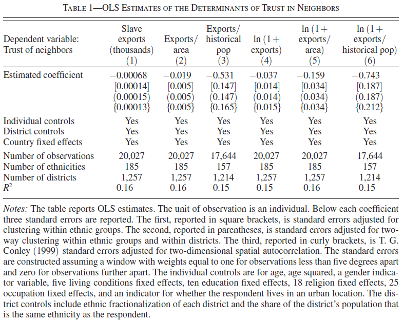
Nunn & Wantchekon 2011, Tab. 1, p.3232

Below, we’ll only reproduce Column 1 that contains the number of slaves taken from an ethnic group (expressed in thousands of people) as measure of the intensity of the slave trade.

# options(scipen=5) # Change display of decimal numbers

# New data object with variable subset
  d2 <- dplyr::select(d, trust_neighbors, exports, age, age2, male,
                      urban_dum, education, occupation, religion,
                      living_conditions, district_ethnic_frac,
                      frac_ethnicity_in_district, isocode,
                      murdock_name, district)
  d2 <- na.omit(d2) # Delete missings - rowwise
  
# Table 1: Trust Relatives (Column 1)
  fit1 <- lm(trust_neighbors ~ exports + age + age2 + male + urban_dum 
             + as.factor(education) + as.factor(occupation) +
               as.factor(religion) + as.factor(living_conditions) +
               district_ethnic_frac + frac_ethnicity_in_district +
               as.factor(isocode), 
             data = d2)
          # as.factor(religion): Add religion as dummy variables
  
# Compute clustered SEs
  SEs <- clx(fit1, 1, d2$murdock_name)
  # SEs
  SEs2way <- mclx(fit1, 1, d2$murdock_name, d2$district)
  # SEs2way
  
# For NERDS? Read Arai (2015) and try using another dfcw 
  # dfcw = degree of freedom correction weight
  # G <- length(unique(d2$murdock_name)) # N of ethnic groups
  # N <- length(d2$murdock_name) # N of individuals
  # dfcw <- (G/(G - 1)) * (N - 1)/fit1$df.residual # df-adjustment
  # clx(fit1, dfcw, d2$murdock_name)
  # mclx(fit1, dfcw, d2$murdock_name, d2$district)

# Include Robust SEs in output
  stargazer(fit1, 
            type = "html", # Output format
            keep = 1, # Only show first independent variable
            se = list(SEs[,2]), # Add own SEs
            omit.stat = "f", # Hide stats
            digits = 5) # Digits in table


	Dependent variable:

	trust_neighbors

exports	-0.00068^***
	(0.00014)


Observations	20,027
R²	0.15583
Adjusted R²	0.15257
Residual Std. Error	0.92749 (df = 19949)

Note:	p<0.1; p<0.05; p<0.01

12.10.5 Table 2, Column 1 and 2

Now let’s have a look at Table 2: OLS Estimates of the Determinants of the Trust of Others (p.3234).

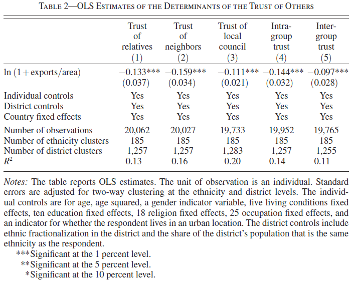
Nunn & Wantchekon 2011, Tab. 2, p.3234

The outcome variables are trust in different categories of people. As above the unit of observation are individuals.

We replicate Table 2 albeit faciliate the task by simply generating one dataset at the beginning and deleting observations listwise, because it facilitates the use of clustered standard errors. For this reason there are slight differences in the estimates we reproduce (see also the difference in N).

# d <- read_dta("https://docs.google.com/uc?id=0Bwer5wQoreiuNkc1cmg0TjFFR1E&export=download")
d2 <- dplyr::select(d,
                    trust_relatives,
                    trust_neighbors,
                    trust_local_council,
                    intra_group_trust,
                    inter_group_trust,
                    ln_export_area, age, age2, male, urban_dum,
                    education, occupation, religion,
                    living_conditions,
                    district_ethnic_frac, frac_ethnicity_in_district, 
                    isocode, murdock_name, district)
  d2 <- na.omit(d2)


  fit1 <- lm(trust_relatives ~ ln_export_area + age + age2 + male +
               urban_dum + as.factor(education) + as.factor(occupation)
             + as.factor(religion) + as.factor(living_conditions) +
               district_ethnic_frac + frac_ethnicity_in_district +
               as.factor(isocode), data = d2)
  fit1.SEs2way <- mclx(fit1, 1, d2$murdock_name, d2$district)
  
  fit2 <- lm(trust_neighbors ~ ln_export_area + age + age2 + male +
               urban_dum + as.factor(education) + as.factor(occupation)
             + as.factor(religion) + as.factor(living_conditions) +
               district_ethnic_frac + frac_ethnicity_in_district +
               as.factor(isocode), data = d2)
  fit2.SEs2way <- mclx(fit2, 1, d2$murdock_name, d2$district)

stargazer(fit1, fit2, 
            type = "html", 
            keep = c("ln_export_area"),
            se = list(fit1.SEs2way[,2],
                      fit2.SEs2way[,2]),
            omit.stat = "f", 
            digits = 5)


	Dependent variable:

	trust_relatives	trust_neighbors
	(1)	(2)

ln_export_area	-0.13528^***	-0.15877^***
	(0.03558)	(0.03318)


Observations	18,397	18,397
R²	0.13036	0.15437
Adjusted R²	0.12670	0.15081
Residual Std. Error (df = 18319)	0.89359	0.92498

Note:	p<0.1; p<0.05; p<0.01

12.10.6 Table 5: IV

Finally, we’ll have a look at the instrumental variable analysis shown in Table 5 (p.3234).

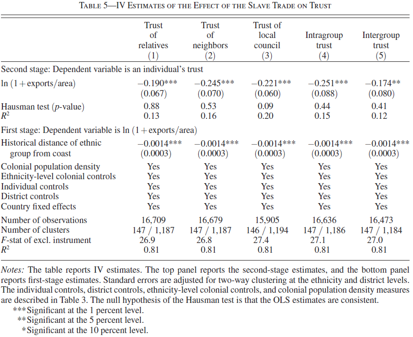
Nunn & Wantchekon 2011, Tab. 5, p.3234

Let’s examine the instrument first.

summary(d$distsea)

Min.	1st Qu.	Median	Mean	3rd Qu.	Max.	NA’s
1.249979	175.3092	393.1697	439.892	675.7052	1252.683	120

d <- read_dta("https://docs.google.com/uc?id=0Bwer5wQoreiuNkc1cmg0TjFFR1E&export=download")
plot_ly(x = d$distsea, type = "histogram") %>%
  layout(xaxis = list(title = 
                        "Historic distance from coast 1000s kms"),
         yaxis = list(title = "Frequency"))

Does the distance to the sea (instrument) affect the number of slave exports (treatment) of particular ethnic groups? Q: Should it?

stargazer(lm(ln_export_area ~ distsea, data=d, na.action=na.omit), 
          type = "html")


	Dependent variable:

	ln_export_area

distsea	-0.001^***
	(0.00002)

Constant	1.107^***
	(0.010)


Observations	21,702
R²	0.184
Adjusted R²	0.184
Residual Std. Error	0.852 (df = 21700)
F Statistic	4,896.528^*** (df = 1; 21700)

Note:	p<0.1; p<0.05; p<0.01

Does the distance to the sea affect current day trust levels? Q: Should it?? What was the intention to treat effect again?

# Character vector with outcome variables
outcome.vars <- c("trust_relatives", "trust_neighbors",
                  "trust_local_council", "intra_group_trust",
                  "inter_group_trust")

# Loop over outcome variables
  for(i in 1:5){

    # Generate model in loop
    model <- paste(outcome.vars[i], " ~ distsea", sep="")
    
    # fit model in loop and create fit objects fit*
    assign(paste("fit", i, sep=""), # assign to new object
           lm(model, data = d, na.action = na.omit)) # fit model
  }
  stargazer(fit1, fit2, fit3, fit4, fit5, type = "html")


	Dependent variable:

	trust_relatives	trust_neighbors	trust_local_council	intra_group_trust	inter_group_trust
	(1)	(2)	(3)	(4)	(5)

distsea	0.0001^***	0.0002^***	0.0004^***	0.0002^***	0.0001^***
	(0.00002)	(0.00002)	(0.00002)	(0.00002)	(0.00002)

Constant	2.145^***	1.659^***	1.467^***	1.568^***	1.321^***
	(0.011)	(0.012)	(0.013)	(0.012)	(0.012)


Observations	20,618	20,580	20,210	20,502	20,301
R²	0.001	0.003	0.016	0.006	0.001
Adjusted R²	0.001	0.003	0.016	0.006	0.001
Residual Std. Error	0.958 (df = 20616)	1.008 (df = 20578)	1.094 (df = 20208)	1.000 (df = 20500)	0.997 (df = 20299)
F Statistic	20.625^*** (df = 1; 20616)	62.243^*** (df = 1; 20578)	326.043^*** (df = 1; 20208)	127.956^*** (df = 1; 20500)	18.415^*** (df = 1; 20299)

Note:	p<0.1; p<0.05; p<0.01

Finally, below we estimate a simple model in which we instrument slave exports with distance to the coast on trust in relatives without any controls.

# See here for a short summary: https://rpubs.com/wsundstrom/t_ivreg
# Instrumental variable regression
  # ivreg(outcome ~ treatment | instrument, data = d)
  # Instrument behind |
 library(AER)
  d2 <- na.omit(d)
  fit <- ivreg(trust_relatives ~ ln_export_area | distsea, 
                  data = d2)
  stargazer(fit, se=list(clx(fit, 1, d2$murdock_name)))

% Table created by stargazer v.5.2.2 by Marek Hlavac, Harvard University. E-mail: hlavac at fas.harvard.edu % Date and time: Tue, May 12, 2020 - 20:00:09

# Classic model
  stargazer(lm(trust_relatives ~ ln_export_area, data = d),
            type="html")


	Dependent variable:

	trust_relatives

ln_export_area	-0.086^***
	(0.007)

Constant	2.235^***
	(0.008)


Observations	20,618
R²	0.007
Adjusted R²	0.007
Residual Std. Error	0.955 (df = 20616)
F Statistic	154.346^*** (df = 1; 20616)

Note:	p<0.1; p<0.05; p<0.01

We can also run some diagnostics. For more info see e.g. here.

## 
## Call:
## ivreg(formula = trust_relatives ~ ln_export_area | distsea, data = d2)
## 
## Residuals:
##     Min      1Q  Median      3Q     Max 
## -2.2315 -0.6338 -0.0690  0.7761  1.6432 
## 
## Coefficients:
##                Estimate Std. Error t value Pr(>|t|)    
## (Intercept)     2.23153    0.01777 125.553  < 2e-16 ***
## ln_export_area -0.23925    0.03104  -7.709 1.46e-14 ***
## 
## Diagnostic tests:
##                   df1  df2 statistic  p-value    
## Weak instruments    1 6577   1171.77  < 2e-16 ***
## Wu-Hausman          1 6576     29.28 6.49e-08 ***
## Sargan              0   NA        NA       NA    
## ---
## Signif. codes:  0 '***' 0.001 '**' 0.01 '*' 0.05 '.' 0.1 ' ' 1
## 
## Residual standard error: 0.9635 on 6577 degrees of freedom
## Multiple R-Squared: -0.01172,    Adjusted R-squared: -0.01188 
## Wald test: 59.42 on 1 and 6577 DF,  p-value: 1.459e-14

And then we try to replicate Column 1 (trust in relatives) and 2 (trust in neighbours) in Table 5 that contains instrumental variable estimates controlling for various covariates.The code below also illustrates how you can loop over a number of outcome variables using the same covariates and generate model fit objects “on the fly”.

# All 5 oucome variable
outcome.vars <- c("trust_relatives", "trust_neighbors")

baseline.controls <- "age + age2 + male + urban_dum + as.factor(education) + as.factor(occupation) + as.factor(religion) + as.factor(living_conditions) + district_ethnic_frac + frac_ethnicity_in_district + as.factor(isocode)"



colonial.controls <- "malaria_ecology + total_missions_area + explorer_contact + railway_contact + cities_1400_dum + as.factor(v30) + v33"




controls <- paste(baseline.controls, " + ", 
                  colonial.controls, 
                  " + ln_init_pop_density", 
                  sep="")

d2 <- d %>% dplyr::select(trust_relatives, trust_neighbors, 
                   ln_export_area, age, 
                  age2, male, urban_dum, distsea,
                  education, occupation, religion, living_conditions,
                  district_ethnic_frac, frac_ethnicity_in_district,
                  isocode, malaria_ecology, total_missions_area,
                  explorer_contact, railway_contact, cities_1400_dum,
                  v30, v33, ln_init_pop_density, murdock_name,
                  district)
d2 <- na.omit(d2)

# Loop: Creates model which is then inserted in the ivreg function.
for(i in 1:2){
  model <- 
    paste(
      outcome.vars[i], 
      " ~ ln_export_area + ", controls, " | ", controls, "+ distsea",
      sep = "")
  # print(model) # show while loop runs
  
    # fit model in loop
    assign(paste("fit", i, sep=""), # assign to new object
           ivreg(model, data = d2))
}

  stargazer(fit1, fit2,
            keep = "ln_export_area",
            se=list(mclx(fit1, 1, d2$murdock_name, d2$district)[,2],
                    mclx(fit2, 1, d2$murdock_name, d2$district)[,2]),
            type = "html", out = "www/iv-table5-col1-col2.html")


	Dependent variable:

	trust_relatives	trust_neighbors
	(1)	(2)

ln_export_area	-0.188^***	-0.244^***
	(0.068)	(0.070)


Observations	16,667	16,667
R²	0.130	0.159
Adjusted R²	0.126	0.155
Residual Std. Error (df = 16575)	0.884	0.911

Note:	p<0.1; p<0.05; p<0.01

References

Arai, Mahmood. 2015. “Cluster-Robust Standard Errors Using R.” Note Available Http://People. Su. Se.

Esarey, Justin. 2016. “Package clusterSEs.”

Esarey, Justin, and Andrew Menger. 2016. “Practical and Effective Approaches to Dealing with Clustered Data.”